horne_extraction
The horne_extraction utility performs an optimal extraction of a source’s flux from an echelle order using the algorithms reported in Horne [Hor86].
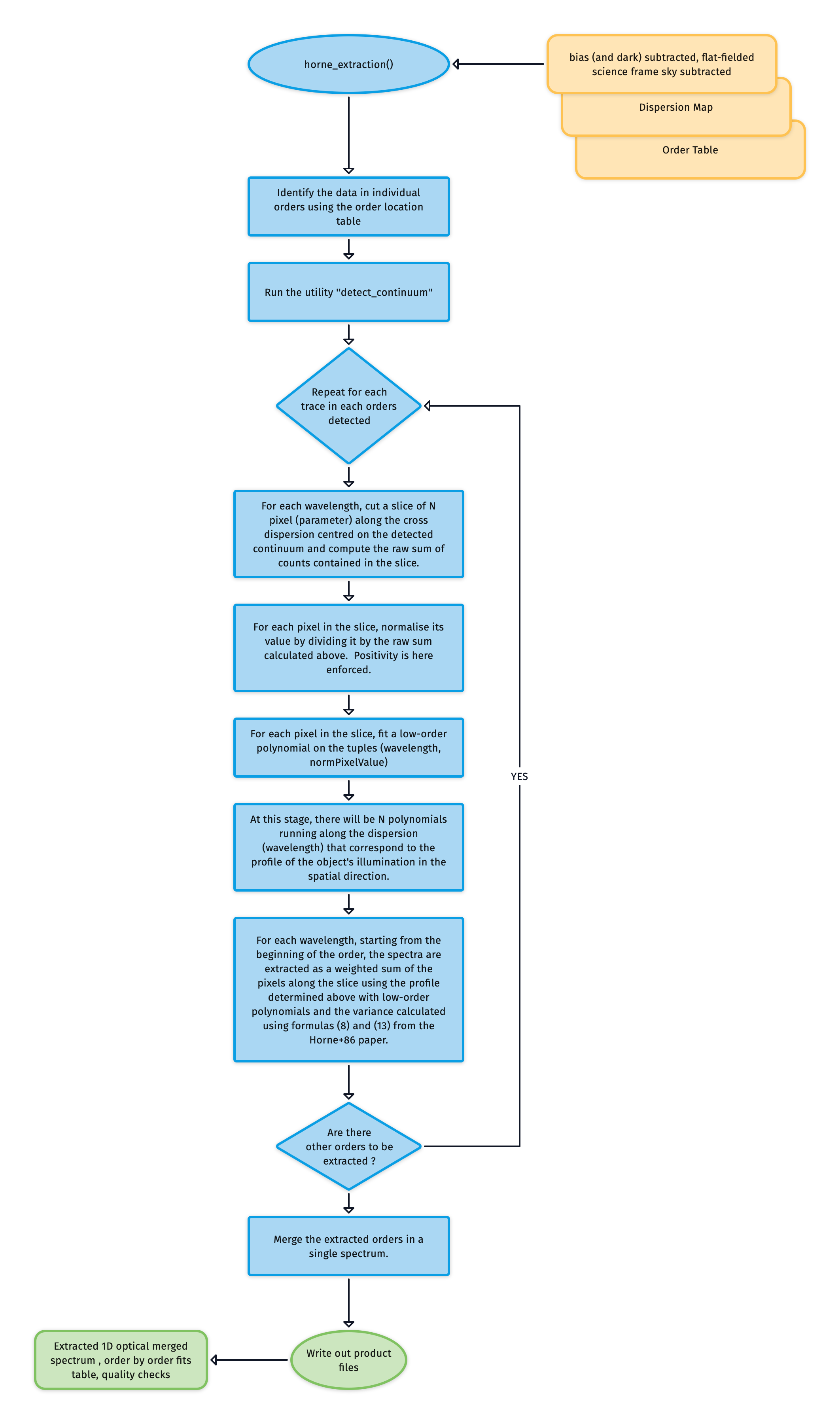
Fig. 70 The algorithm used to optimally extract an object spectrum.
This utility, according to the prescription of Horne [Hor86], follows those basic steps:
1 Determination of the spatial profile
Starting from the order_table computed by the detect_continumm utility, the horne_extraction utility runs along the spectral direction and takes, for each wavelength centred in the position measured by the detect_continuum utility, a window of 1xhorne-extraction-slit-length. Then, the pixels are summed, and each pixel in the slice is normalized as
where N = horne-extraction-slit-length.
The flux is normalised for each cross-dispersion slice to detect the object’s profile. Then, multiple parallel polynomials are fitted, and outliers are removed using an iterative fitting procedure. Bad pixels are masked. The final flux for each cross-dispersion slide is a weighted sum, as reported in Horne, with the bad pixels and outliers accounted for.
Then, a low-order polynomial is fitted for each pixel in the slice (multiple parallel polynomials), modelling the value of the fractional flux received along the dispersion axis. During the iterative fitting procedure, bad pixels are masked and outliers (CRHs etc) are removed. The complete set of polynomials represents the object’s profile along the spatial direction for each wavelength. For a slice length of N pixels, there will be N different polynomials, one per pixel.
Polynomials are fitted with subsequent iterations. Pixels for which residuals deviate more than the horne-extraction-profile-clipping-sigma standard deviation are removed before attempting a new fitting of the data. The procedure is repeated for a maximum of horne-extraction-profile-clipping-iteration-count times.
When the procedure above is completed, the actual extraction occurs as follows:
2 Extraction of the spectrum for each wavelength for each order.
Using the polynomials computed above, the extracted integrated flux for each wavelength in the order is calculated as follows:
Where \(P_{i}^{\lambda}\) is the value of the polynomial for the pixel \(i^{th}\) evaluated at wavelength \(\lambda\), \(D_{i}^{\lambda}\) is the raw pixel value on the 2D image, detrended and sky subtracted, of the science object and \(S_{i}^{\lambda}\) is the estimated value, at the same pixel position, of the 2D image of the sky model computed in stare mode. When this utility is applied to nodding or offset mode images, this value is chosen to be zero. \(V_{i}^{\lambda}\) is the so-called variance image and is computed as
Where \(V_{0}\) is the square of the readout noise of the detector, \(f_{\lambda}\) is the sum of the pixels within the extraction window at each wavelength, and \(Q\) is the detector gain.
Cosmic rays and uncorrected deviant pixels are removed from the extraction by comparing their value with a certain threshold. In particular, for each pixel \(i\) in the extraction window the quantity
is computed. The extraction does not include pixels for which this quantity exceeds the horne-extraction-profile-global-clipping-sigma.
The final flux for each cross-dispersion slice is a weighted sum, as reported in Horne [Hor86], with the bad pixels and outliers accounted for. Note, if more than 3 bad/outlying pixels are found within a cross-dispersion slice, then the slice is ignored.
3 Merging of spectral orders
The spectrum is extracted on each order separately. When all orders are extracted, they are merged together in a single spectrum. Since regions of different orders overlap in the wavelength space, they are first rectified on a common, equally spaced wavelength grid in order to merge together. Flux during resampling is conserved.
Utility API
- class horne_extraction(log, settings, recipeSettings, skyModelFrame, skySubtractedFrame, unflattenedFrame, twoDMapPath, recipeName=False, qcTable=False, productsTable=False, dispersionMap=False, sofName=False, locationSetIndex=False, startNightDate='', notFlattened=False, debug=False, turnOffMP=False)[source]
Bases:
objectperform optimal source extraction using the Horne method (Horne 1986)
Key Arguments:
log– loggersettings– the settings dictionaryrecipeSettings– the recipe specific settingsskyModelFrame– path to sky model frameskySubtractedFrame– path to sky subtracted frameunflattenedFrame– path to unflattened frametwoDMapPath– path to 2D dispersion map image pathrecipeName– name of the recipe as it appears in the settings dictionaryqcTable– the data frame to collect measured QC metricsproductsTable– the data frame to collect output products (if False no products are saved to file)dispersionMap– the FITS binary table containing dispersion map polynomialsofName– the set-of-files filenamelocationSetIndex– the index of the AB cycle locations (nodding mode only). Default FalsestartNightDate– YYYY-MM-DD date of the observation night. Default “”notFlattened– flag to indicate if the frame is flattened or not. Default Falsedebug– flag to indicate if debug mode is on (shows plots). Default FalseturnOffMP– turn off multiprocessing. True or False. Default False. If True, multiprocessing will be turned off and the recipe will run in serial. This is useful for debugging.
Usage:
To setup your logger, settings and database connections, please use the
fundamentalspackage (see tutorial here https://fundamentals.readthedocs.io/en/master/initialisation.html).To initiate a horne_extraction object, use the following:
from soxspipe.commonutils import horne_extraction
optimalExtractor = horne_extraction(
    log=log,
    skyModelFrame=skyModelFrame,
    skySubtractedFrame=skySubtractedFrame,
    unflattenedFrame=unflattenedFrame,
    twoDMapPath=twoDMap,
    settings=settings,
    recipeName="soxs-stare",
    qcTable=qc,
    productsTable=products,
    dispersionMap=dispMap,
    sofName=sofName,
    locationSetIndex=locationSetIndex,
    startNightDate=startNightDate,
    debug=debug,
    turnOffMP=turnOffMP

)
qc, products = optimalExtractor.extract()
Initialization
- extract()[source]
extract the full spectrum order-by-order and return FITS Binary table containing order-merged spectrum
Return:
qcTable– the data frame to collect measured QC metricsproductsTable– the data frame to collect output productsmergedSpectumDF– path to the FITS binary table containing the merged spectrum
- merge_extracted_orders(extractedOrdersDF)[source]
merge the extracted order spectra in one continuous spectrum
Key Arguments:
extractedOrdersDF– a data-frame containing the extracted orders
Return:
None