response_function

The response_function utility computes the spectrograph’s response function, using an observation of a suitable bright standard star. The function computed by this utility is used to flux calibrate the scientific spectra, converting from ADU to \(erg\) \(cm^{-2} s^{-1} A^{-1}\).

The general algorithm and steps performed by response_function are reported in the Fig. 73.

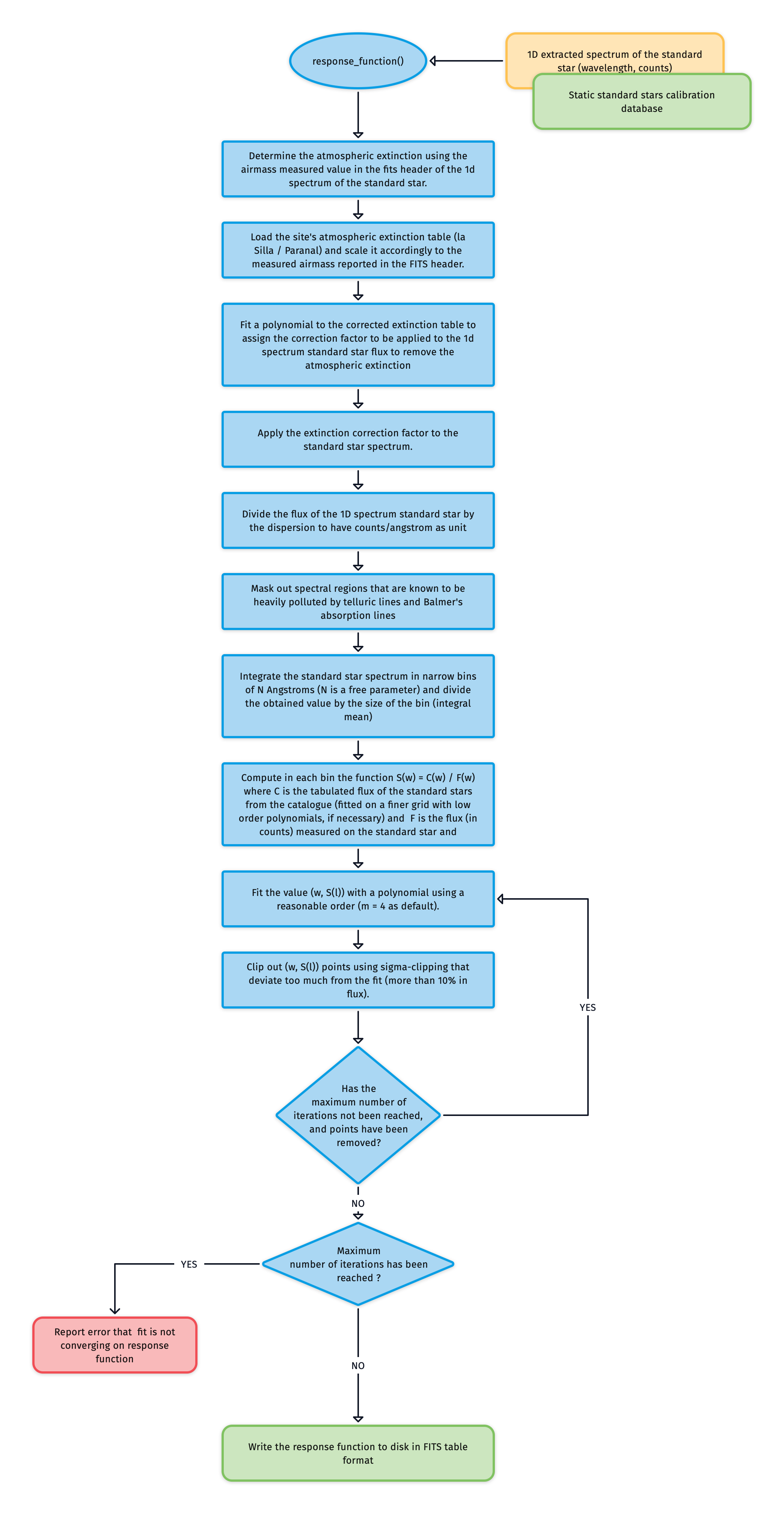
Fig. 73 The algorithm used to compute the spectrograph’s response function.

In detail, this utility first determines the average airmass at which the standard star, provided as input, has been observed. Then, it loads the standard extinction curve, supplied as a FITS table with wavelength and \(mag_{airmass}\) for the observing site (La Silla for NTT/SOXS), and corrects the observed flux (in counts) accordingly, applying the formula:

\[ fluxCorrected_{\lambda} = fluxObserved_{\lambda} \times 10^{AM \times mag_{airmass}} \]

Please note that the tabulated extinction curve and the observed spectrum are fitted with a nearest-neighbour interpolation schema to cope with the different discretisations.

The \(fluxCorrected_{\lambda}\) values are then converted in \(ADU\) \({A}^{-1} s^{-1}\) by diving for the value contained in the EXPTIME keyword of the standard star spectrum and for the dispersion measured at each pixel. According to the considered arm (UV-VIS, NIR), regions that are known to be polluted by significant telluric absorptions or strong Lyman or Balmer/Paschen lines are masked out.

The observed standard star spectrum is then averaged in narrow bins of about 10 \(A\) to increase the signal-to-noise ratio (a sort of narrow-band photometry). Then, from the tabulated value of the standard star catalogue (interpolated on a suitable grid), the function:

\[ S(\lambda) \propto \frac{C(\lambda)}{F(\lambda)} \]

where \(C(\lambda)\) is the tabulated value of the standard star flux in the catalogue (in \(erg\) \(cm^{-2} s^{-1} A^{-1}\)), and \(F(\lambda)\) is the flux (in ADU) measured on the standard star.

The different values of \(S(\lambda)\) are fitted with a polynomial of 4th order (as default) or soxs-response-poly_order using a standard iteration schema. For each iteration, data are fitted, and points for which the residuals deviate more soxs-response-sigma_clipping_threshold standard deviations are clipped for the next iteration (with a maximum of soxs-response-max_iteration number of iterations).

If the fit does not converge, response_function raises an exception; otherwise, a FITS table containing the fit’s parameters is saved.

Efficiency Calculation

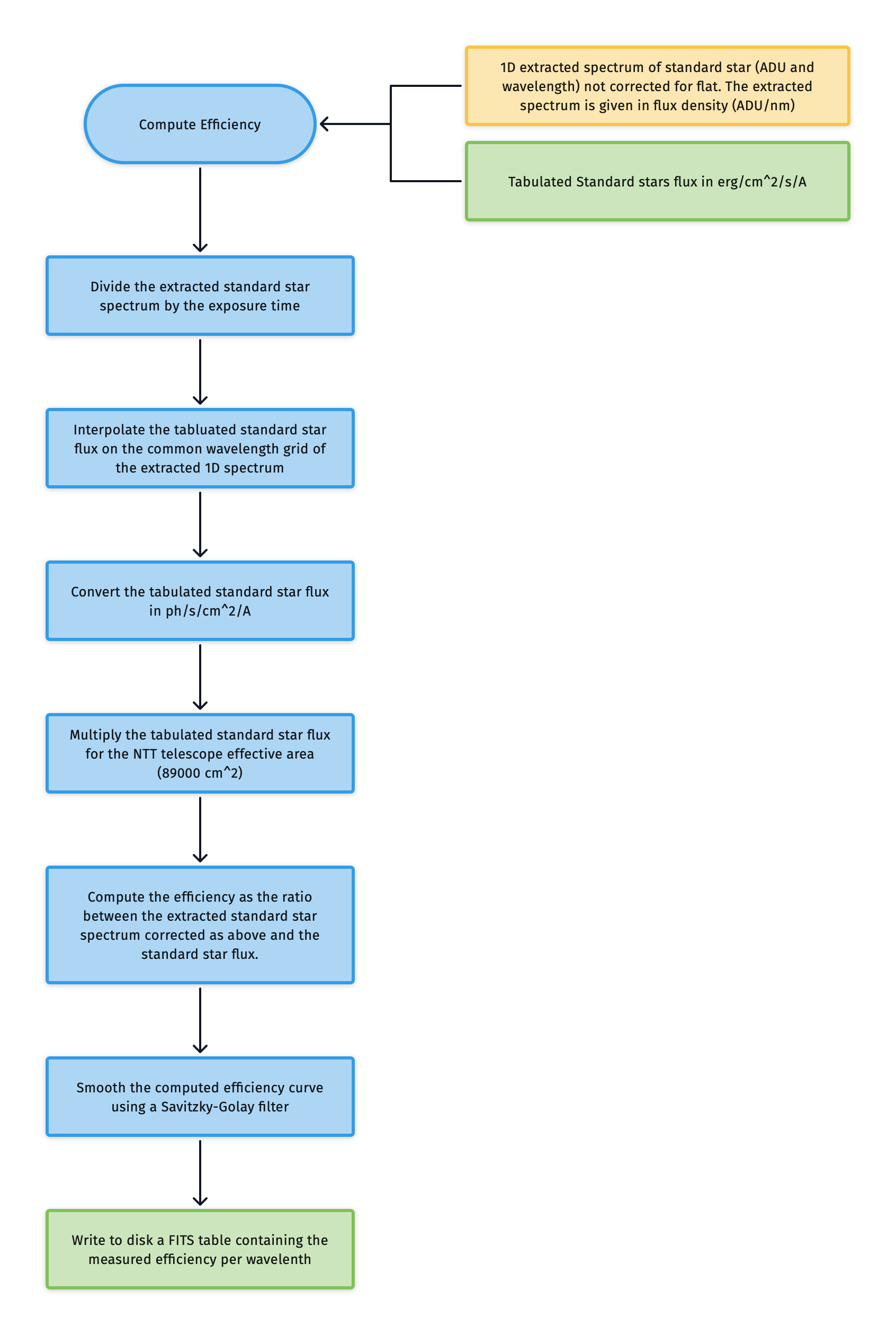
Fig. 74 The algorithm used to compute the telescope and instrument efficiency.

During the computation of the response function, the get() method performs an evaluation of the efficiency of the instrument as the ratio between the measured counts from the observed and not flat field corrected standard star spectrum and the expected number of counts from tabulated flux values of known standard stars.

In detail, the get() method searches the FITS header for the standard name to load the tabulated expected flux value from the static calibration assets for the observed standard star. It then divides the observed spectrum by the exposure time (EXPTIME keyword in the FITS header) and reinterpolates the tabulated standard star fluxes onto the same wavelength grid as the observed spectrum. The tabulated flux values are then converted into ph s\(^{-1} cm^{-2} \AA^{-1}\) and multiplied by the effective NTT telescope area (89,000 cm\(^2\)). Finally, the observed standard star spectrum is divided by the tabulated standard star fluxes (adjusted as discussed above) to obtain the estimate of the end-to-end efficiency, which is smoothed using a standard Savitzky-Golay filter with \(\sigma\) = 21.

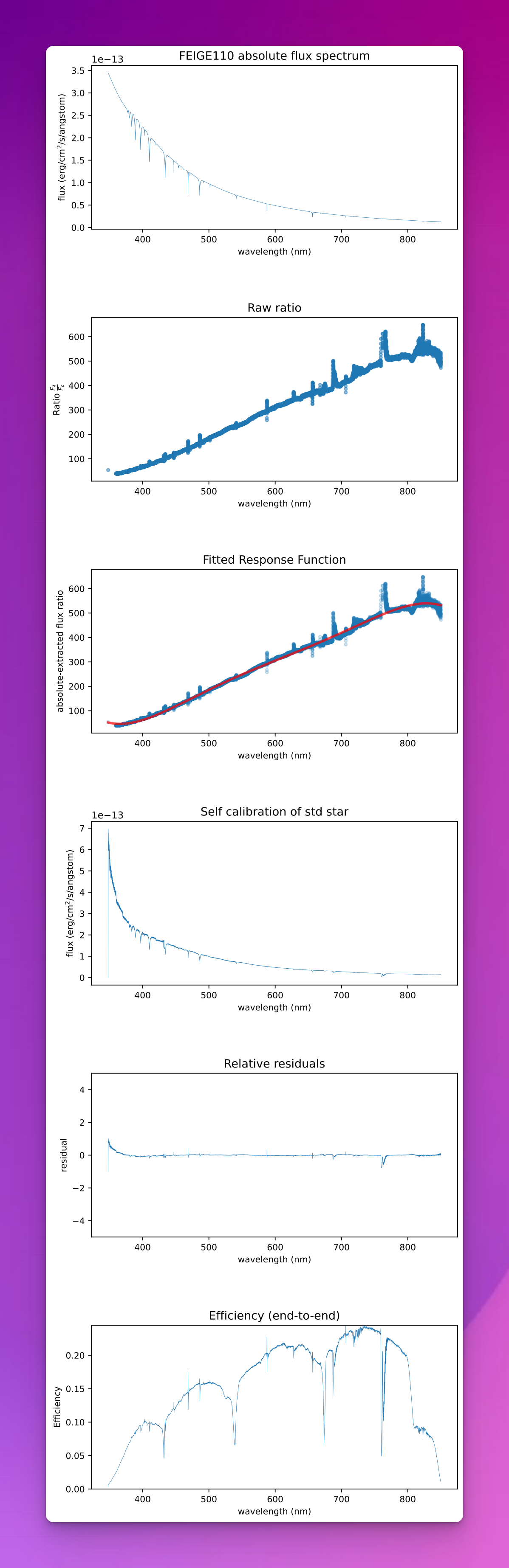
Fig. 75 The output of the reponse_function utility used in the reduction of spectroscopic standard star spectra. The third panel shows th fittted response curve, and the final panel shows the overall efficiency of the instrument across the entire wavelength range of the spectrograph arm.

Utility API

class response_function(log, stdExtractionPath, recipeName, sofName, settings=False, qcTable=False, productsTable=False, startNightDate='', stdNotFlatExtractionPath='', orderJoins=None)

Bases: object

Given a standard star extracted spectrum, generate the instrument response function needed to flux calibrate science spectra

Key Arguments: - log – logger - settings – the settings dictionary - stdExtractionPath – fits binary table containing the extracted standard spectrum - recipeName – name of the recipe as it appears in the settings dictionary - settings – the pipeline settings - sofName – name of the originating SOF file - qcTable – the data frame to collect measured QC metrics - productsTable – the data frame to collect output products - startNightDate – YYYY-MM-DD date of the observation night. Default “” - stdNotFlatExtractionPath – fits binary table containing the extracted standard spectrum without flat correction. Default “”. - orderJoins – a list of tuples indicating the orders to be joined together in the response function fitting. Default None.

Usage:

To setup your logger, settings and database connections, please use the fundamentals package (see tutorial here <http://fundamentals.readthedocs.io/en/latest/#tutorial>_).

To initiate a response_function object, use the following:

from soxspipe.commonutils import response_function
response = response_function(
    log=log,
    settings=settings,
    recipeName=recipeName,
    sofName=sofName,
    stdExtractionPath=stdExtractionPath
    qcTable=qcTable,
    productsTable=productsTable,
    startNightDate=startNightDate
    stdNotFlatExtractionPath=stdNotFlatExtractionPath,
    orderJoins=orderJoins,
)
qcTable, productsTable = response.get()

Initialization

get()

get the response_function object

Return: - response_function – a set of polynomial coefficients

plot_response_curve(stdExtWave, stdExtWaveNotFlat, stdExtFlux, binCentreWave, binCentreWaveOriginal, binIntegratedFlux, absToExtFluxRatio, responseFuncCoeffs, stdEfficiencyEstimate)

generate a QC plot for the response curve

Key Arguments:

• stdExtWave – the extracted standard star wavelength

• stdExtFlux – the extracted standard star flux

• stdExtWaveNotFlat – the extracted standard star wavelength (not flattened)

• binCentreWave – binned wavelengths after clipping (during fitting)

• binCentreWaveOriginal – binned wavelengths

• binIntegratedFlux – binned flux

• absToExtFluxRatio – the ratio of the absolute flux vs the extraction flux

• responseFuncCoeffs – the response function coefficients

• stdEfficiencyEstimate – the estimated instrument efficiency

Return: - plotFilePath – the path to the QC plot PDF

write_response_function_to_file(responseFuncCoeffs, polyOrder)

write out the fitted polynomial solution coefficients to file

Key Arguments:

• responseFuncCoeffs – the response curve coefficients

• polyOrder – the order of polynomial used to fit the curve

Return:

• responseCurvePath – path to the saved file