subtract_sky

The subtract_sky utility uses the on-frame data provided in a two-dimensional spectral image to accurately model the sky background, which is removed from the original data frame.

The Kelson Background Subtraction method, initially outlined in Kelson [Kel03], attempts to make optimal use of all data provided in a two-dimensional spectral image to accurately model a sky background image, which can then be removed from the original data frame. The method allows sky-subtraction to be performed in the early stages of the data-reduction process (just after flat-fielding) with no need first to identify and isolate cosmic-ray hits or other bad-pixel values.

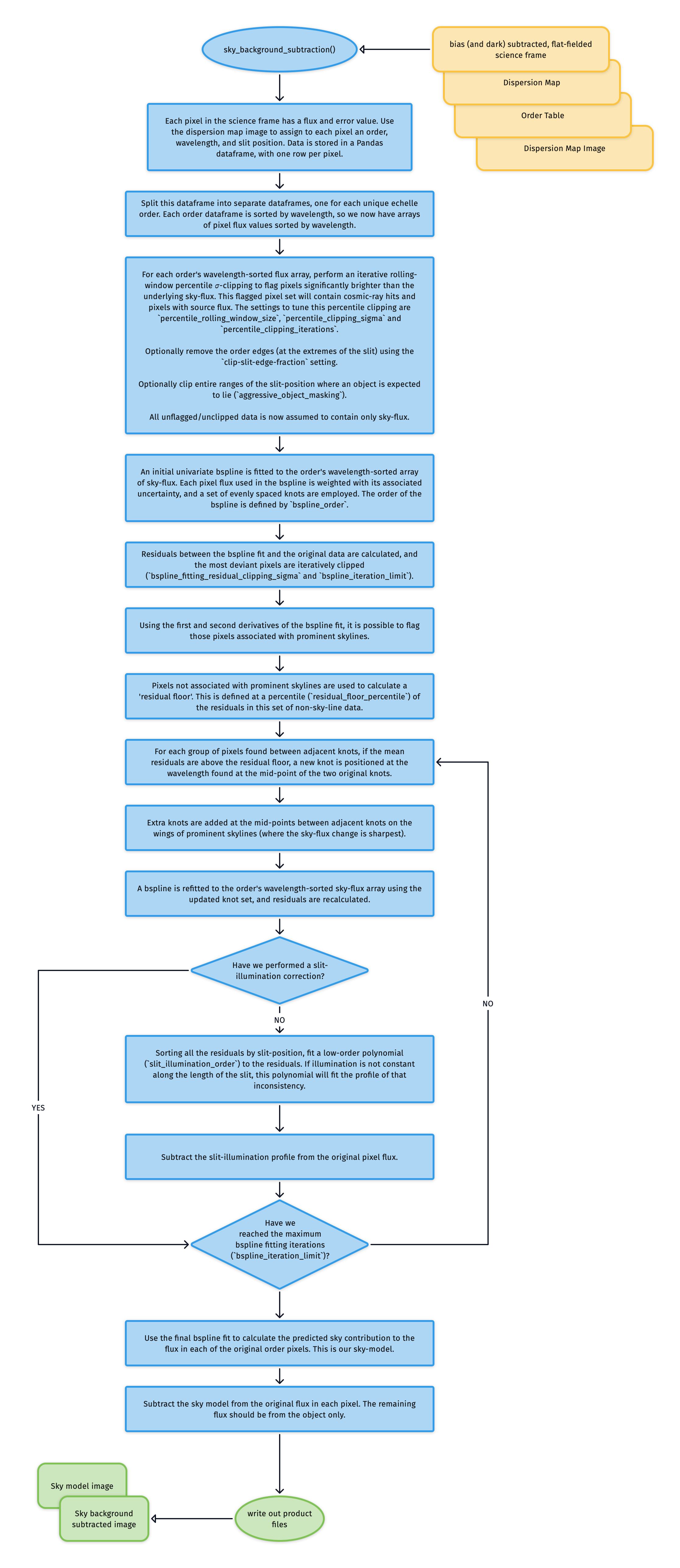
Fig. 81 The algorithm used to model and subtract the sky-flux from data taken in stare mode.

Due to the curved format of each order (at least in the SOXS NIR data) and the cross-dispersion tilt of the skylines, each pixel measures flux at a slightly different wavelength to its neighbours. This provides us with an over-sampled spectrum of the sky.

The first step is to assign a wavelength, slit position and echelle order number to each detector pixel via the 2D dispersion map. Next, we flatten the data for each order to provide the over-sampled, wavelength-sorted flux array.

An iterative rolling-window percentile smoothing with 𝜎-clipping flags pixels significantly brighter than the underlying sky flux (see Fig. 82 and Fig. 83). These flagged pixels will contain cosmic-ray hits and pixels with source flux. Fig. 84 shows the locations of these flagged pixels on the original detector plane; the trace of the object has been successfully masked. The settings to tune this percentile clipping are percentile_rolling_window_size, percentile_clipping_sigma, and percentile_clipping_iterations.

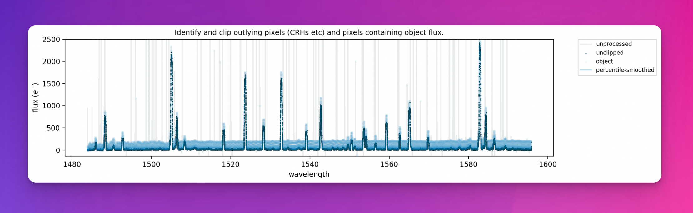
Fig. 82 The narrow spikes seen in the original data (grey) represent the cosmic ray hits and other bad-pixel values contaminating our measurements of the background night sky. The blue line is the percentile smoothed data (a close approximation to the sky spectrum), and the faint blue crosses are pixels flagged as containing flux other than just the sky.

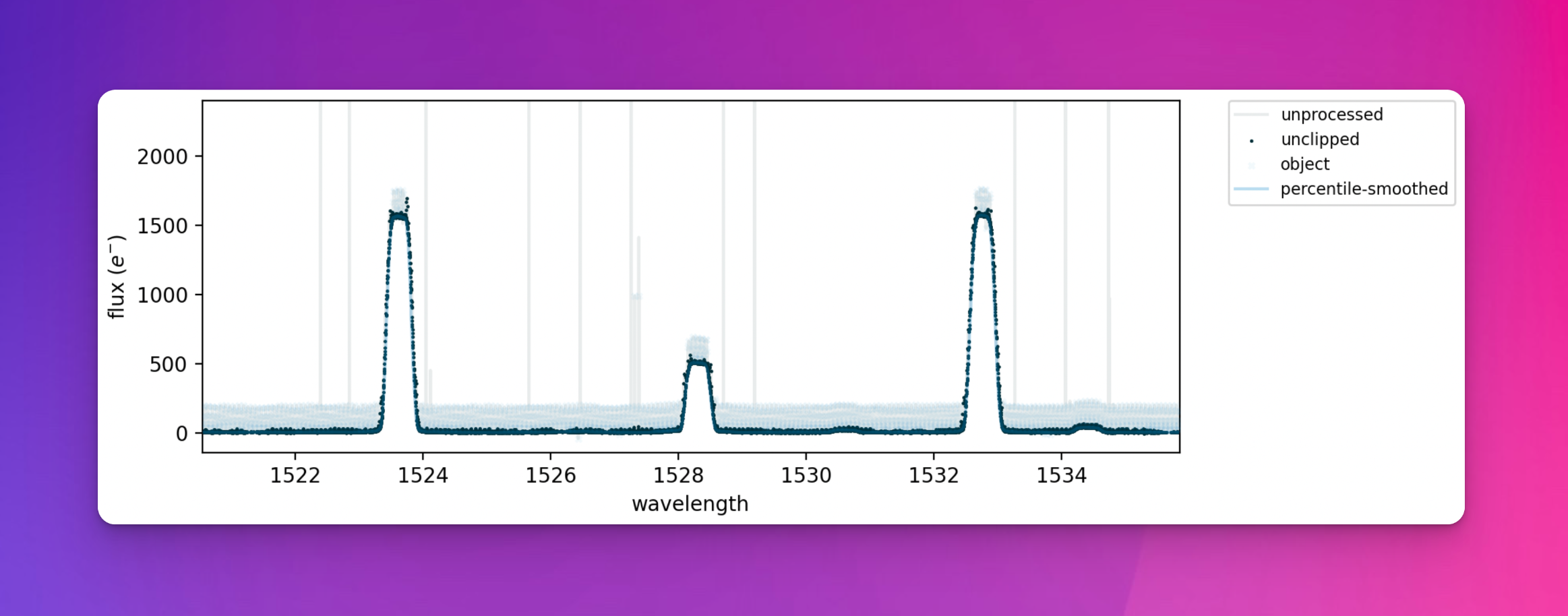
Fig. 83 A zoom of the figure above. Pixels containing object flux are seen to contain flux above the background sky.

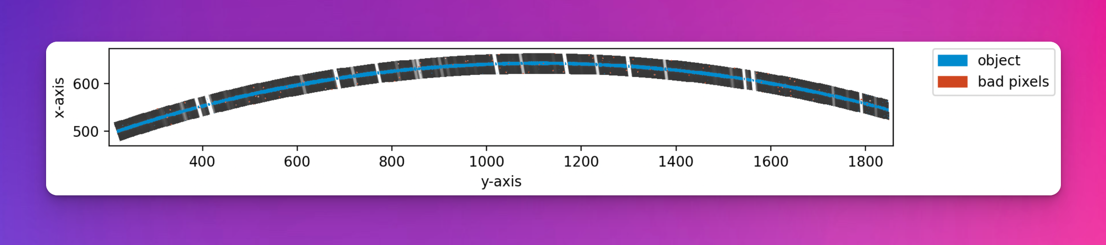
Fig. 84 The original echelle order with pixels flagged as containing object flux or cosmic-ray hits marked in blue.

Next, an initial univariate bspline is fitted to the order’s wavelength-sorted array of sky-flux (with contaminated pixels removed). Each pixel flux used in the bspline is weighted with its associated uncertainty, and a set of evenly spaced knots are employed. The order of the bspline is defined by bspline_order. Residuals between the bspline fit and the original data are calculated, and the most deviant pixels are iteratively clipped (bspline_fitting_residual_clipping_sigma and bspline_iteration_limit).

Using the first and second derivatives of the bspline fit, those pixels associated with prominent skylines are flagged. Pixels not associated with prominent skylines are used to calculate a ‘residual floor’. This is defined at a percentile (residual_floor_percentile) of the residuals in this set of non-sky-line data. For each group of pixels found between adjacent knots, if the mean residuals are above the residual floor, a new knot is positioned at the wavelength found at the mid-point of the two original knots. Extra knots are also added at the mid-points between adjacent knots on the wings of prominent skylines (where the sky-flux change is sharpest).

A bspline is refitted to the order’s wavelength-sorted sky-flux array using the updated knot set, and residuals are recalculated.

At this stage, all the residuals are sorted by slit-position, and a low-order polynomial with order slit_illumination_order is fitted to the residuals. If illumination is not constant along the length of the slit, this polynomial will fit the profile of that inconsistency. This slit illumination profile is subtracted from the original pixel flux.

A final round of iterative bspline fitting is performed, each time adding new knots at locations where the residuals exceed the residual floor determined earlier and at the wings of prominent skylines. This continues until the bspline fitting iteration limit (bspline_iteration_limit) is reached. Fig. 85 shows the final bspline fit that is used as the sky model.

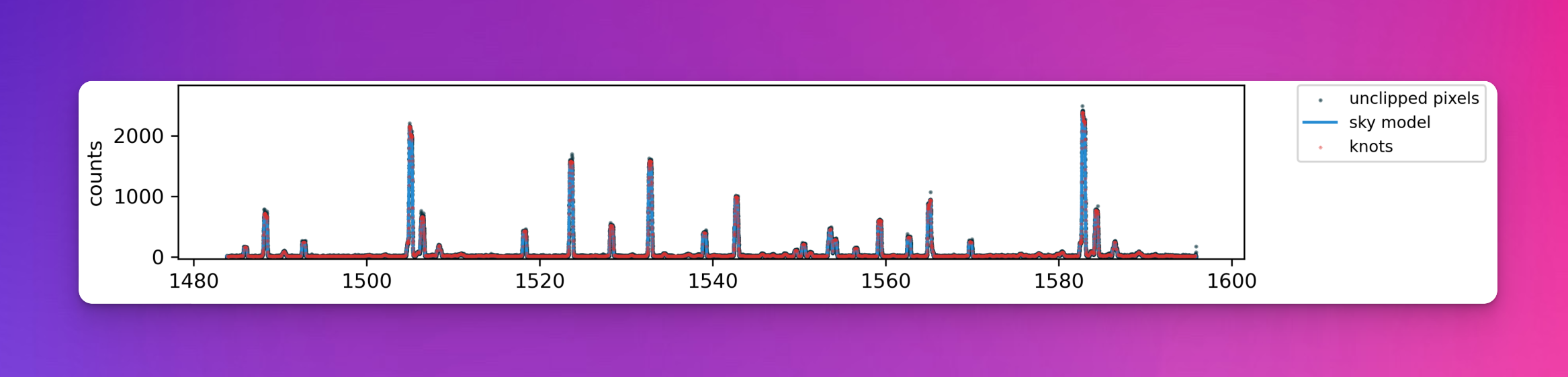
Fig. 85 A bspline fit of the sky spectrum. The black dots are the sky flux values coming from individual pixels, the red diamonds are the strategically placed knot, and the blue line is the final bspline fit to the data (the sky model).

Finally, this bspline fit is used to generate an estimation of the sky flux level in every pixel in the original detector space (top panel of Fig. 86), which is then subtracted from the original image to produce a sky-subtracted frame ready for object extraction.

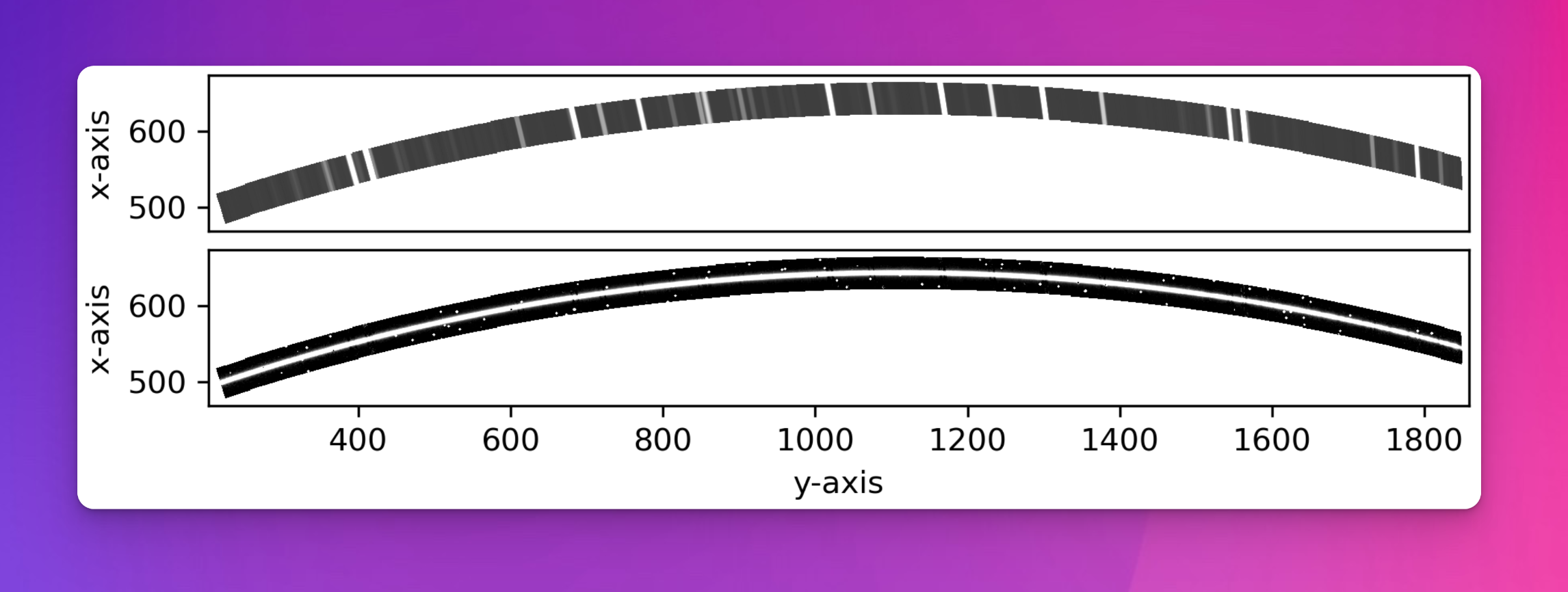
Fig. 86 The bspline fit is used to estimate the sky flux level in every pixel in the original detector space (top panel), which is then subtracted from the original image to produce a frame with the sky removed (bottom panel). The object trace can be clearly seen now the skylines have been removed.

Utility API

class subtract_sky(log, settings, recipeSettings, objectFrame, twoDMap, qcTable, productsTable, dispMap=False, sofName=False, recipeName='soxs-stare', startNightDate='', debug=False)

Bases: object

Subtract the sky background from a science image using the Kelson Method

A model of the sky-background is created using a method similar to that described in Kelson, D. (2003), Optimal Techniques in Two-dimensional Spectroscopy: Background Subtraction for the 21st Century (http://dx.doi.org/10.1086/375502). This model-background is then subtracted from the original science image to leave only non-sky flux.

Key Arguments:

• log – logger

• settings – the soxspipe settings dictionary

• recipeSettings – the recipe specific settings

• objectFrame – the image frame in need of sky subtraction

• twoDMap – 2D dispersion map image path

• qcTable – the data frame to collect measured QC metrics

• productsTable – the data frame to collect output products

• dispMap – path to dispersion map. Default False

• sofName – name of the originating SOF file. Default False

• recipeName – name of the recipe as it appears in the settings dictionary. Default soxs-stare

• startNightDate – YYYY-MM-DD date of the observation night. Default “”

Usage:

To setup your logger and settings, please use the fundamentals package (see tutorial here https://fundamentals.readthedocs.io/en/master/initialisation.html).

To initiate a subtract_sky object, use the following:

from soxspipe.commonutils import subtract_sky
skymodel = subtract_sky(
    log=log,
    settings=settings,
    recipeSettings=recipeSettings,
    objectFrame=objectFrame,
    twoDMap=twoDMap,
    qcTable=qc,
    productsTable=products,
    dispMap=dispMap
)
skymodelCCDData, skySubtractedCCDData, qcTable, productsTable = skymodel.subtract()

Initialization

add_data_to_placeholder_images(imageMapOrderDF, skymodelCCDData, skySubtractedCCDData, skySubtractedResidualsCCDData)

add sky-model and sky-subtracted data to placeholder images

Key Arguments:

• imageMapOrderDF – single order dataframe from object image and 2D map

• skymodelCCDData – the sky model

• skySubtractedCCDData – the sky-subtracted data

Usage:

self.add_data_to_placeholder_images(imageMapOrderSkyOnly, skymodelCCDData, skySubtractedCCDData)

adjust_tilt(orderDF, tck)

correct the tilt of the slit by attempting to minimise the residuals of the bspline fit while shifting the tilt angle

Key Arguments:

• orderDF – a single order dataframe containing sky-subtraction flux residuals used to determine and remove a slit-illumination correction

• tck – spline parameters to replot

Return:

• orderDF – dataframe with wavelengths adjusted for a corrected tilt

Usage:

orderDF = self.adjust_tilt(orderDF, tck)

calculate_residuals(skyPixelsDF, fluxcoeff, orderDeg, wavelengthDeg, slitDeg, writeQCs=False)

calculate residuals of the polynomial fits against the observed line positions

Key Arguments:

• skyPixelsDF – the predicted line list as a data frame

• fluxcoeff – the flux-coefficients

• orderDeg – degree of the order fitting

• wavelengthDeg – degree of wavelength fitting

• slitDeg – degree of the slit fitting (False for single pinhole)

• writeQCs – write the QCs to dataframe? Default False

Return:

• residuals – combined x-y residuals

• mean – the mean of the combine residuals

• std – the stdev of the combine residuals

• median – the median of the combine residuals

clip_object_slit_positions(order_dataframes, aggressive=False)

clip out pixels flagged as an object

Key Arguments:

• order_dataframes – a list of order data-frames with pixels potentially containing the object flagged.

Return:

• order_dataframes – the order dataframes with the object(s) slit-ranges clipped

• sky_only_dataframes – dataframes with object removed

Usage:

allimageMapOrder = self.clip_object_slit_positions(
    allimageMapOrder,
    aggressive=True
)

create_placeholder_images()

create placeholder images for the sky model and sky-subtracted frame

Return:

• skymodelCCDData – placeholder for sky model image

• skySubtractedCCDData – placeholder for sky-subtracted image

Usage:

skymodelCCDData, skySubtractedCCDData = self.create_placeholder_images()

cross_dispersion_flux_normaliser(orderDF)

measure and normalise the flux in the cross-dispersion direction

Key Arguments:

• orderDF – a single order dataframe containing sky-subtraction flux residuals used to determine and remove a slit-illumination correction

Return:

• correctedOrderDF – dataframe with slit-illumination correction factor added (flux-normaliser)

Usage:

correctedOrderDF = self.cross_dispersion_flux_normaliser(orderDF)

determine_residual_floor(imageMapOrder, tck, iteration)

determine residual floor and flag sky-lines

Key Arguments: - imageMapOrderDF – dataframe with various processed data for a given order - tck – the fitted bspline components. t for knots, c of coefficients, k for order - iteration – the iteration number of the sky-subtraction loop, used to determine how aggressive to be in flagging sky-lines and determining the residual floor

Return:

• imageMapOrder – same dataframe but now with sky-line locations flagged

• residualFloor – the residual floor determined within regions containing no skylines.

Usage:

imageMapOrder, residualFloor = self.determine_residual_floor(imageMapOrder, tck)

fit_bspline_curve_to_sky(imageMapOrder)

fit a single-order univariate bspline to the unclipped sky pixels (wavelength vs flux)

Key Arguments:

• imageMapOrder – single order dataframe, containing sky flux with object(s) and CRHs removed

• order – the order number

Return:

• imageMapOrder – same imageMapOrder as input but now with sky_model (bspline fit of the sky) and sky_subtracted_flux columns

• tck – the fitted bspline components. t for knots, c of coefficients, k for order

Usage:

imageMapOrder, tck = self.fit_bspline_curve_to_sky(
    imageMapOrder
)

get_over_sampled_sky_from_order(imageMapOrder, clipBPs=True, clipSlitEdge=False)

unpack the over sampled sky from an order

Key Arguments:

• imageMapOrder – single order dataframe from object image and 2D map

• clipBPs – clip bad-pixels? Default True

• clipSlitEdge – clip the slit edges. Percentage of slit width to clip. Default False

Return:

• imageMapOrder – input order dataframe with outlying pixels masked AND object pixels masked

Usage:

imageMapOrderWithObject, imageMapOrderSkyOnly = skymodel.get_over_sampled_sky_from_order(imageMapOrder, o, ignoreBP=False, clipSlitEdge=0.00)

plot_image_comparison(objectFrame, skyModelFrame, skySubFrame)

generate a plot of original image, sky-model and sky-subtraction image

Key Arguments:

• objectFrame – object frame

• skyModelFrame – sky model frame

• skySubFrame – sky subtracted frame

Return:

• filePath – path to the plot pdf

plot_order_skymodel_fitting_quicklook(imageMapOrder, tck, title=None, knots=False)

Quick-look diagnostic plot of the sky-model fit for a single order.

plot_sky_sampling(order, imageMapOrderDF, tck=False, knotLocations=False)

generate a plot of sky sampling

Key Arguments:

• order – the order number.

• imageMapOrderDF – dataframe with various processed data for order

• tck – spline parameters to replot

• knotLocations – wavelength locations of all knots used in the fit

Return:

• filePath – path to the generated QC plots PDF

Usage:

self.plot_sky_sampling(
    order=myOrder,
    imageMapOrderDF=imageMapOrder
)

rolling_window_clipping(imageMapOrderDF, windowSize, sigma_clip_limit=5, max_iterations=10)

clip pixels in a rolling wavelength window

Key Arguments:

• imageMapOrderDF – dataframe with various processed data for a given order

• windowSize – the window-size used to perform rolling window clipping (number of data-points)

• sigma_clip_limit – clip data values straying beyond this sigma limit. Default 5

• max_iterations – maximum number of iterations when clipping

Return:

• imageMapOrderDF – image order dataframe with ‘clipped’ == True for those pixels that have been clipped via rolling window clipping

Usage:

imageMapOrder = self.rolling_window_clipping(
    imageMapOrderDF=imageMapOrder,
    windowSize=23,
    sigma_clip_limit=4,
    max_iterations=10
)

subtract()

generate and subtract a sky-model from the input frame

Return:

• skymodelCCDData – CCDData object containing the model sky frame

• skySubtractedCCDData – CCDData object containing the sky-subtracted frame

• qcTable – the data frame containing measured QC metrics

• productsTable – the data frame containing collected output products