create_dispersion_map

The create_dispersion_map utility searches for emission line detections in arc-lamp frames imaged through pinhole masks. The measured line positions are then iteratively fitted with a set of polynomials to produce a global dispersion solution (and spatial solution in the case of a multi-pinhole frame). Both the soxs_disp_solution and soxs_spatial_solution recipes use the utility. The final wavelength solution is provided in air.

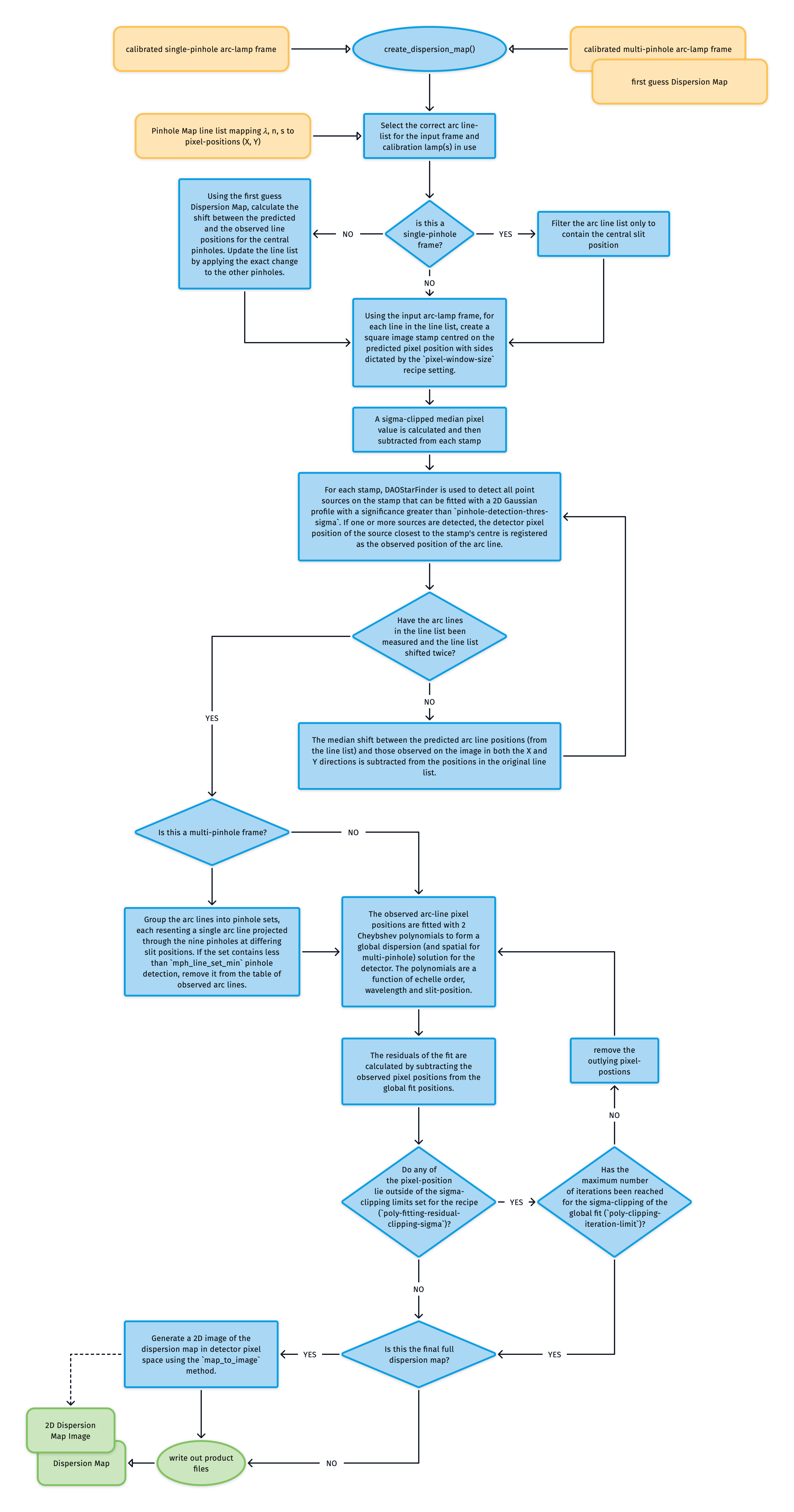
Fig. 55 This algorithm fits a dispersion solution to the SOXS or Xshooter spectral arms via calibration arc-lamp frames taken with single and multi-pinhole masks.

The pipeline’s static calibration suite contains arc line lists listing the wavelength \(\lambda\), order number \(n\) and slit position \(s\) of arc lamp spectral lines alongside a first approximation of their (\(X, Y\)) pixel positions on the detector.

If the input arc frame was taken through the single-pinhole mask, the line list is filtered to contain just the central pinhole positions. If, however, the input is a multi-pinhole frame, then the first guess Dispersion Map (created with soxs_disp_solution) is used to calculate the shift between the predicted and observed line positions for the central pinholes. The pixel positions for the entire line list are updated by applying the same pixel shift to the other pinholes.

For each line in the line list:

• An image stamp centred on the predicted pixel position (\(X_o, Y_o\)) of dimensions winX and winY is generated from the pinhole calibration frame.

• A sigma-clipped median pixel value is calculated and subtracted from each stamp.

• DAOStarFinder is employed to search for the observed detector position (\(X, Y\)) of the arc line via 2D Gaussian profile fitting on the stamp (see Fig. 56).

• The bad-pixel mask is considered when measuring the position of the pinhole arc-line and if a lines falls on a bad-pixel it is ignored.

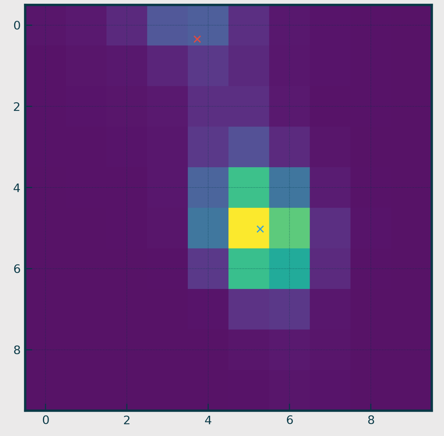
Fig. 56 One of the stamps cut from a pinhole-masked arc-lamp frame. The stamp is selected using a window centred around the predicted pixel position of an arc line (read from the static calibration arc line list table). DAOStarFinder is then used to search for point-like sources on the stamp. In this stamp, two sources were found (each marked by an ‘x’), with the source closest to the stamp’s centre (blue ‘x’) chosen as the observed location of the arc line.

We now have a list of arc-line wavelengths, their observed pixel positions, and the order in which they were detected. These values are used to iteratively fit two polynomials that describe the detector’s global dispersion solution. In the case of the single-pinhole frames, these are:

\[X = \sum\limits_{ij} c_{ij} \times n^i \times \lambda^j\]

\[Y = \sum\limits_{ij} c_{ij} \times n^i \times \lambda^j\]

where \(\lambda\) is wavelength and \(n\) is the echelle order number.

In the case of the multi-pinhole, we also have the slit position \(s\), and so add a spatial solution to the dispersion solution:

\[X = \sum\limits_{ijk} c_{ijk} \times n^i \times \lambda^j \times s^k\]

\[Y = \sum\limits_{ijk} c_{ijk} \times n^i \times \lambda^j \times s^k\]

Upon each iteration, the residuals between the fits and the measured pixel positions are calculated, and sigma-clipping is employed to eliminate measurements that stray too far from the fit. Once the maximum number of iterations is reached or all outlying lines have been clipped, the coefficients of the polynomials are written to a Dispersion map file.

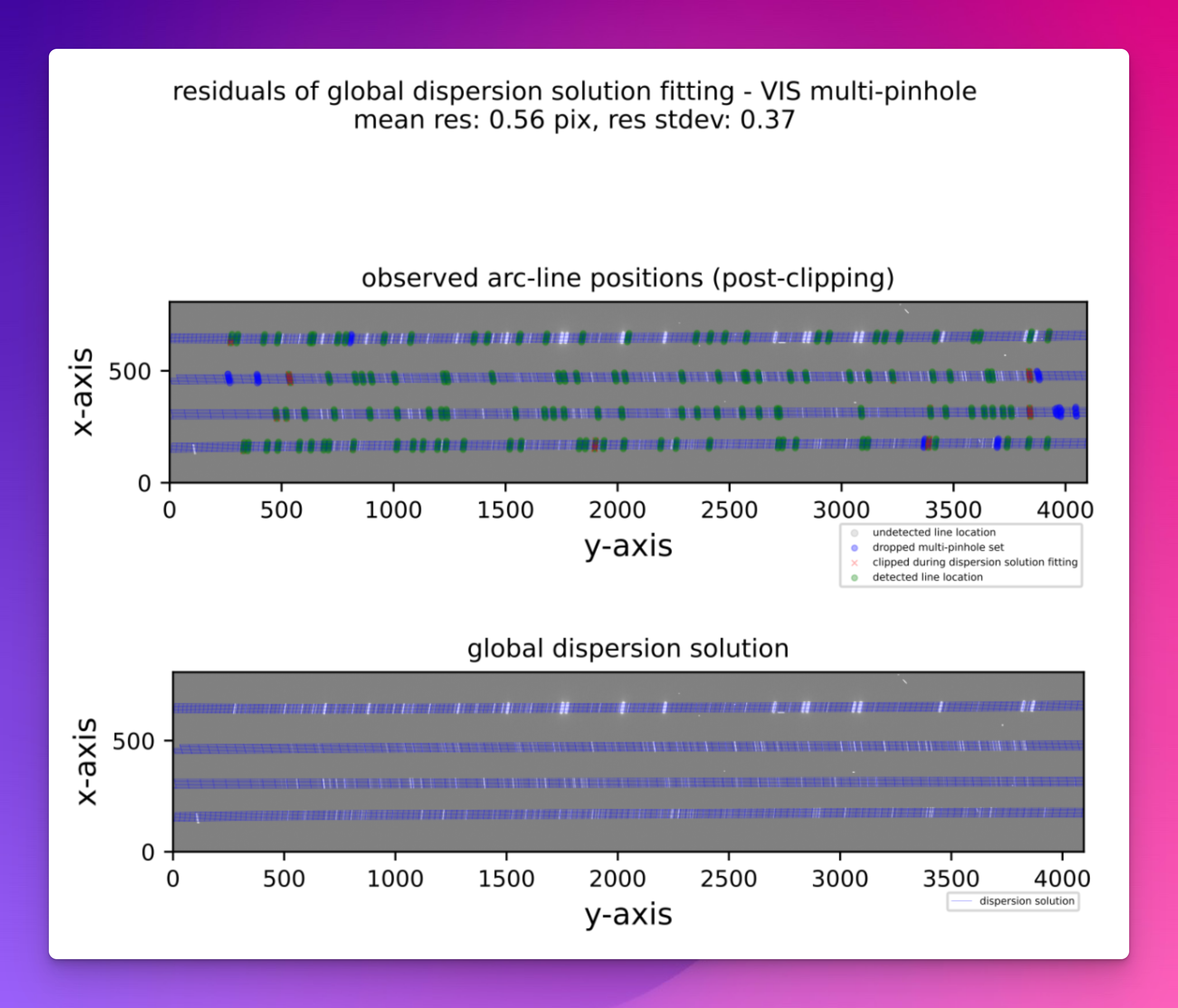
Fig. 57 A QC plot resulting from the soxs_spatial_solution recipe. The top panel shows a SOXS VIS arc-lamp frame, taken with a multi-pinhole mask. The green circles represent arc lines detected in the image, and the blue circles and red crosses are lines that were detected but dropped because other pinholes of the same arc line were not detected, or because the lines were clipped during polynomial fitting. The grey circles represent arc lines reported in the static calibration table that were not detected in the image. The bottom panel shows the same arc-lamp frame with the dispersion solution overlaid as a blue grid. Lines travelling along the dispersion axis (left to right) are lines of equal slit position, and lines travelling in the cross-dispersion direction (top to bottom) are lines of equal wavelength.

2D Image Map

The Dispersion map is used to generate a triple-extension FITS file with each extension image exactly matching the dimensions of the detector (see Fig. 59). The first extension contains the wavelength value at the centre of each pixel location, the second the slit position, and the third the order number. The solutions for these images are iteratively converged in a brute-force manner (see Fig. 58}). These image maps are used in sky-background subtraction and object extraction utilities.

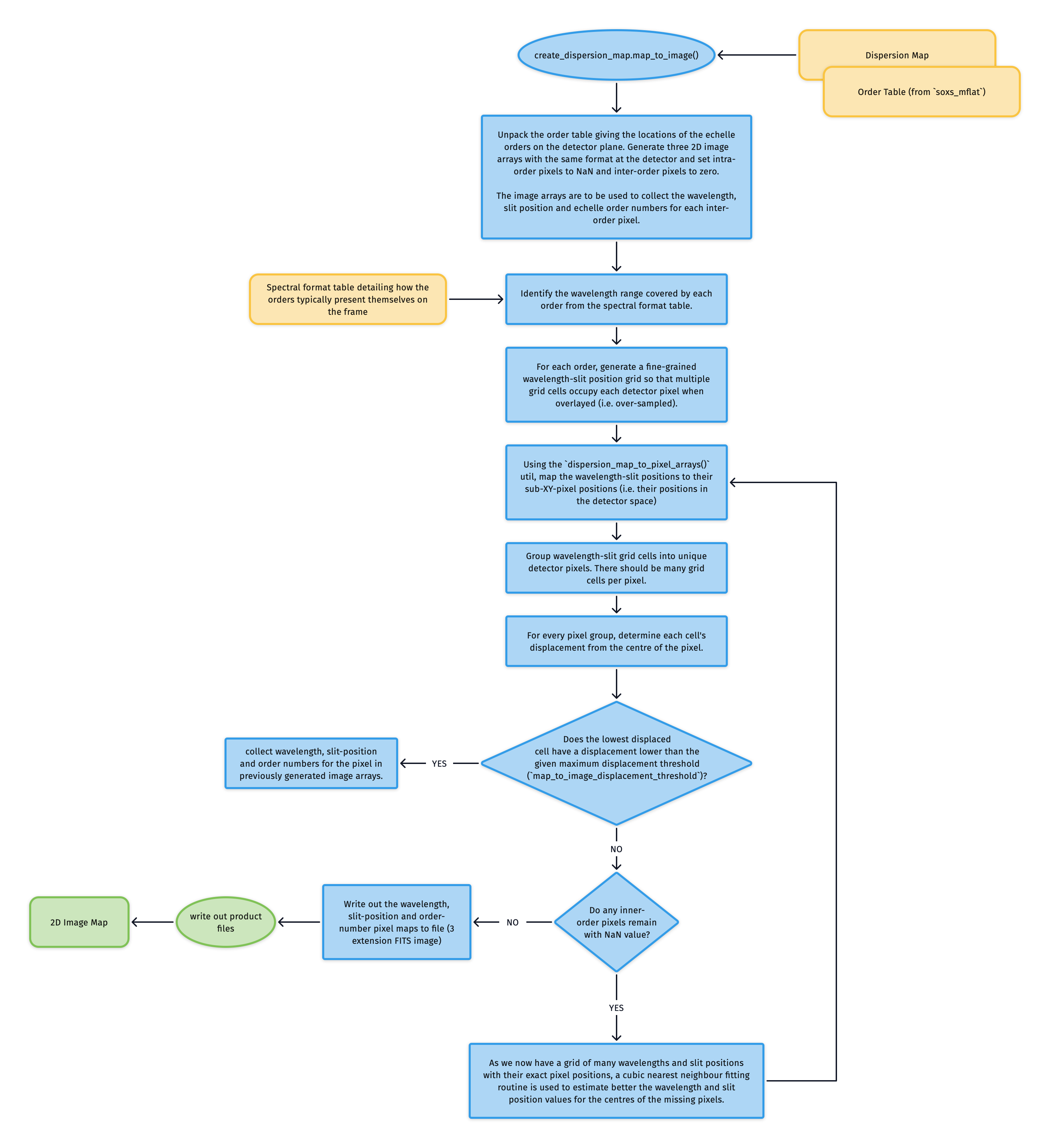
Fig. 58 This is the algorithm used to transform the dispersion solution into a 2D image map, with individual FITS extensions for wavelength, slit position, and order number.

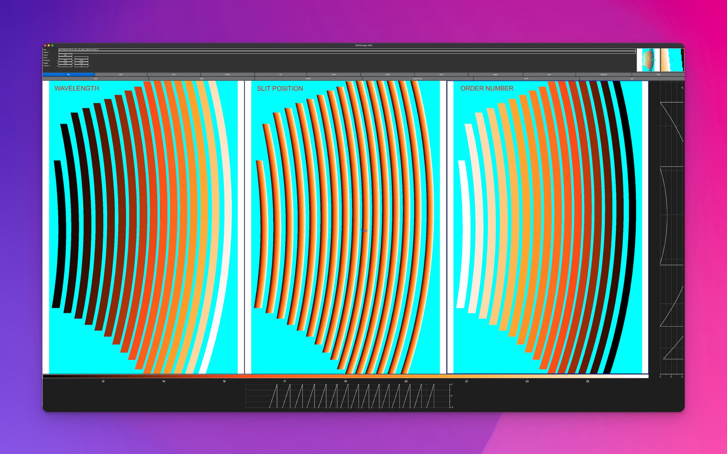
Fig. 59 A 2D dispersion solution image map; a triple-extension FITS file with each extension image exactly matching the dimensions of the detector. The first extension contains the wavelength value at the centre of each pixel location, the second the slit position, and the third the order number.

Utility API

class create_dispersion_map(log, settings, recipeSettings, pinholeFrame, firstGuessMap=False, orderTable=False, qcTable=False, productsTable=False, sofName=False, create2DMap=True, lineDetectionTable=False, startNightDate='', arcFrame=None, debug=False, turnOffMP=False)

Bases: object

detect arc-lines on a pinhole frame to generate a dispersion solution

Key Arguments:

• log – logger

• settings – the settings dictionary

• recipeSettings – the recipe specific settings

• pinholeFrame – the calibrated pinhole frame (single or multi)

• firstGuessMap – the first guess dispersion map from the soxs_disp_solution recipe (needed in soxs_spat_solution recipe). Default False.

• orderTable – the order geometry table

• qcTable – the data frame to collect measured QC metrics

• productsTable – the data frame to collect output products

• sofName – name of the originating SOF file

• create2DMap – create the 2D image map of wavelength, slit-position and order from disp solution.

• lineDetectionTable – the list of arc-lines detected on the pinhole frame (used only for pipeline tuning)

• startNightDate – YYYY-MM-DD date of the observation night. Default “”

• arcFrame – the calibrated arc frame used to determine spectral resolution. Default None

• debug – debug mode. Default False

• turnOffMP – turn off multiprocessing. Default False.

Usage:

from soxspipe.commonutils import create_dispersion_map
mapPath, mapImagePath, res_plots, qcTable, productsTable = create_dispersion_map(
    log=log,
    settings=settings,
    pinholeFrame=frame,
    firstGuessMap=False,
    qcTable=self.qc,
    productsTable=self.products,
    sofName=sofName,
    create2DMap=True,
    recipeSettings=recipeSettings,
    startNightDate=startNightDate,
    arcFrame=arcFrame,
    debug=debug,
    turnOffMP=turnOffMP
).get()

Initialization

calculate_residuals(orderPixelTable, xcoeff, ycoeff, orderDeg, wavelengthDeg, slitDeg, writeQCs=False, pixelRange=False)

calculate residuals of the polynomial fits against the observed line positions

Key Arguments:

• orderPixelTable – the predicted line list as a data frame

• xcoeff – the x-coefficients

• ycoeff – the y-coefficients

• orderDeg – degree of the order fitting

• wavelengthDeg – degree of wavelength fitting

• slitDeg – degree of the slit fitting (False for single pinhole)

• writeQCs – write the QCs to dataframe? Default False

• pixelRange – return centre pixel and ± 2nm from the centre pixel (to measure the pixel scale)

Return:

• residuals – combined x-y residuals

• mean – the mean of the combine residuals

• std – the stdev of the combine residuals

• median – the median of the combine residuals

convert_and_fit(order, bigWlArray, bigSlitArray, slitMap, wlMap, iteration, plots=False)

convert wavelength and slit position grids to pixels

Key Arguments:

• order – the order being considered

• bigWlArray – 1D array of all wavelengths to be converted

• bigSlitArray – 1D array of all split-positions to be converted (same length as bigWlArray)

• slitMap – place-holder image hosting fitted pixel slit-position values

• wlMap – place-holder image hosting fitted pixel wavelength values

• iteration – the iteration index (used for CL reporting)

• plots – show plot of the slit-map

Return:

• orderPixelTable – dataframe containing unfitted pixel info

• remainingCount – number of remaining pixels in orderTable

Usage:

orderPixelTable = self.convert_and_fit(
        order=order, bigWlArray=bigWlArray, bigSlitArray=bigSlitArray, slitMap=slitMap, wlMap=wlMap)

create_new_static_line_list(dispersionMapPath)

using a first pass dispersion solution, use a line atlas to generate a more accurate and more complete static line list

Key Arguments:

• dispersionMapPath – path to the first pass dispersion solution

Return:

• newPredictedLineList – a new predicted line list (to replace the static calibration line-list)

create_placeholder_images(order=False, plot=False, reverse=False)

create CCDData objects as placeholders to host the 2D images of the wavelength and spatial solutions from dispersion solution map

Key Arguments:

• order – specific order to generate the placeholder pixels for. Inner-order pixels set to nan, else set to 0. Default False (generate all orders)

• plot – generate plots of placeholder images (for debugging). Default False.

• reverse – Inner-order pixels set to 0, else set to nan (reverse of default output).

Return:

• slitMap – placeholder image to add pixel slit positions to

• wlMap – placeholder image to add pixel wavelength values to

Usage:

slitMap, wlMap, orderMap = self._create_placeholder_images(order=order)

detect_pinhole_arc_lines(orderPixelTable, iraf=True, sigmaLimit=3, iteration=False, brightest=False, exclude_border=False, returnAll=False)

detect the observed position of an arc-line given the predicted pixel positions

Key Arguments:

• orderPixelTable – the initial line list

• iraf – use IRAF star finder to generate a FWHM

• sigmaLimit – the lower sigma limit for arc line to be considered detected

• iteration – which detect and shift iteration are we on?

• brightest – find the brightest source?

• exclude_border – exclude border pixels from detection?

Return:

• predictedLine – the line with the observed pixel coordinates appended (if detected, otherwise nan)

fit_polynomials(orderPixelTable, wavelengthDeg, orderDeg, slitDeg, missingLines=False)

iteratively fit the dispersion map polynomials to the data, clipping residuals with each iteration

Key Arguments:

• orderPixelTable – data frame containing order, wavelengths, slit positions and observed pixel positions

• wavelengthDeg – degree of wavelength fitting

• orderDeg – degree of the order fitting

• slitDeg – degree of the slit fitting (0 for single pinhole)

• missingLines – lines not detected on the image

Return:

• xcoeff – the x-coefficients post clipping

• ycoeff – the y-coefficients post clipping

• goodLinesTable – the fitted line-list with metrics

• clippedLinesTable – the lines that were sigma-clipped during polynomial fitting

get()

generate the dispersion map

Return:

• mapPath – path to the file containing the coefficients of the x,y polynomials of the global dispersion map fit

Workflow:

1. LOAD PREDICTED LINE POSITIONS FROM CALIBRATION FILES

2. PREPARE PINHOLE FRAME (MASKING, STATISTICS)

3. ITERATIVELY DETECT ARC LINES ON FRAME

4. FIT POLYNOMIAL DISPERSION SOLUTION

5. WRITE OUTPUTS (LINE LISTS, MAP FILES, QC PLOTS)

get_predicted_line_list()

lift the predicted line list from the static calibrations

Return:

• orderPixelTable – a panda’s data-frame containing wavelength,order,slit_index,slit_position,detector_x,detector_y

map_to_image(dispersionMapPath, orders=False)

convert the dispersion map to images in the detector format showing pixel wavelength values and slit positions

Key Arguments:

• dispersionMapPath – path to the full dispersion map to convert to images

• orders – orders to add to the image map. List. Default False (add all orders)

Return:

• dispersion_image_filePath – path to the FITS image with an extension for wavelength values and another for slit positions

Usage:

mapImagePath = self.map_to_image(dispersionMapPath=mapPath)

order_to_image(orderInfo)

convert a single order in the dispersion map to wavelength and slit position images

Key Arguments:

• orderInfo – tuple containing the order number to generate the images for, the minimum wavelength to consider (from format table) and maximum wavelength to consider (from format table).

Return:

• slitMap – the slit map with order values filled

• wlMap – the wavelengths map with order values filled

Usage:

slitMap, wlMap = self.order_to_image(order=order,minWl=minWl, maxWl=maxWl)

update_static_line_list_detector_positions(originalOrderPixelTable, dispersionMapPath)

using a first pass dispersion solution, update the original static line list

Key Arguments:

• originalOrderPixelTable – original order pixel table

• dispersionMapPath – path to the first pass dispersion solution

Return:

• updatedLineList – updated static line list

write_map_to_file(xcoeff, ycoeff, orderDeg, wavelengthDeg, slitDeg)

write out the fitted polynomial solution coefficients to file

Key Arguments:

• xcoeff – the x-coefficients

• ycoeff – the y-coefficients

• orderDeg – degree of the order fitting

• wavelengthDeg – degree of wavelength fitting

• slitDeg – degree of the slit fitting (False for single pinhole)

Return:

• disp_map_path – path to the saved file