detect_continuum

The detect_continuum utility locates and fits a trace using a low-level polynomial across all echelle orders.

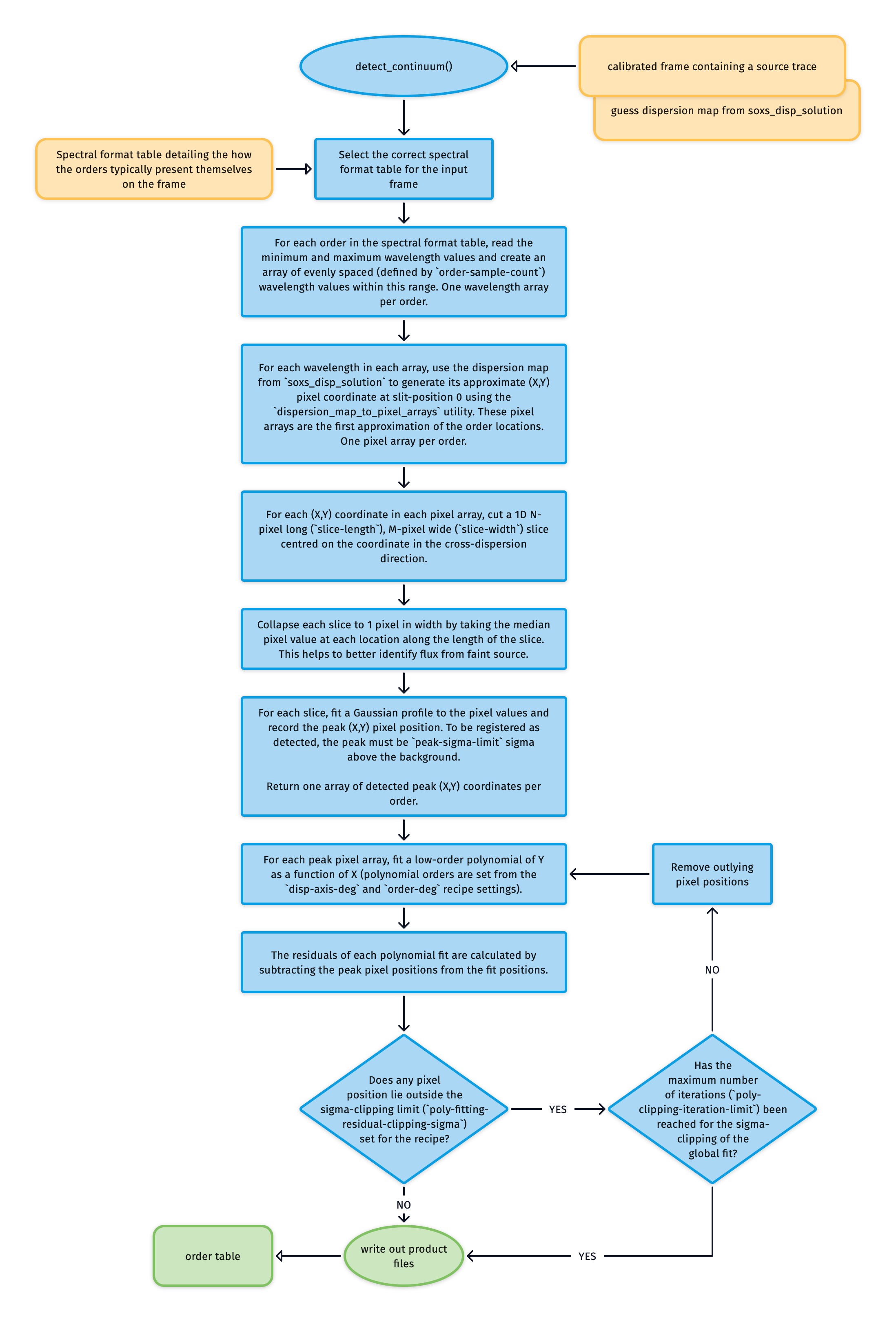
Fig. 60 The algorithm used to fit a source trace across all the echelle orders.

The detect_continuum utility takes an image frame containing a source trace as input. This trace could be from a calibration lamp (as used in the soxs-order-centres recipe, see Fig. 61) or an astrophysical object; the algorithm to fit the trace is the same.

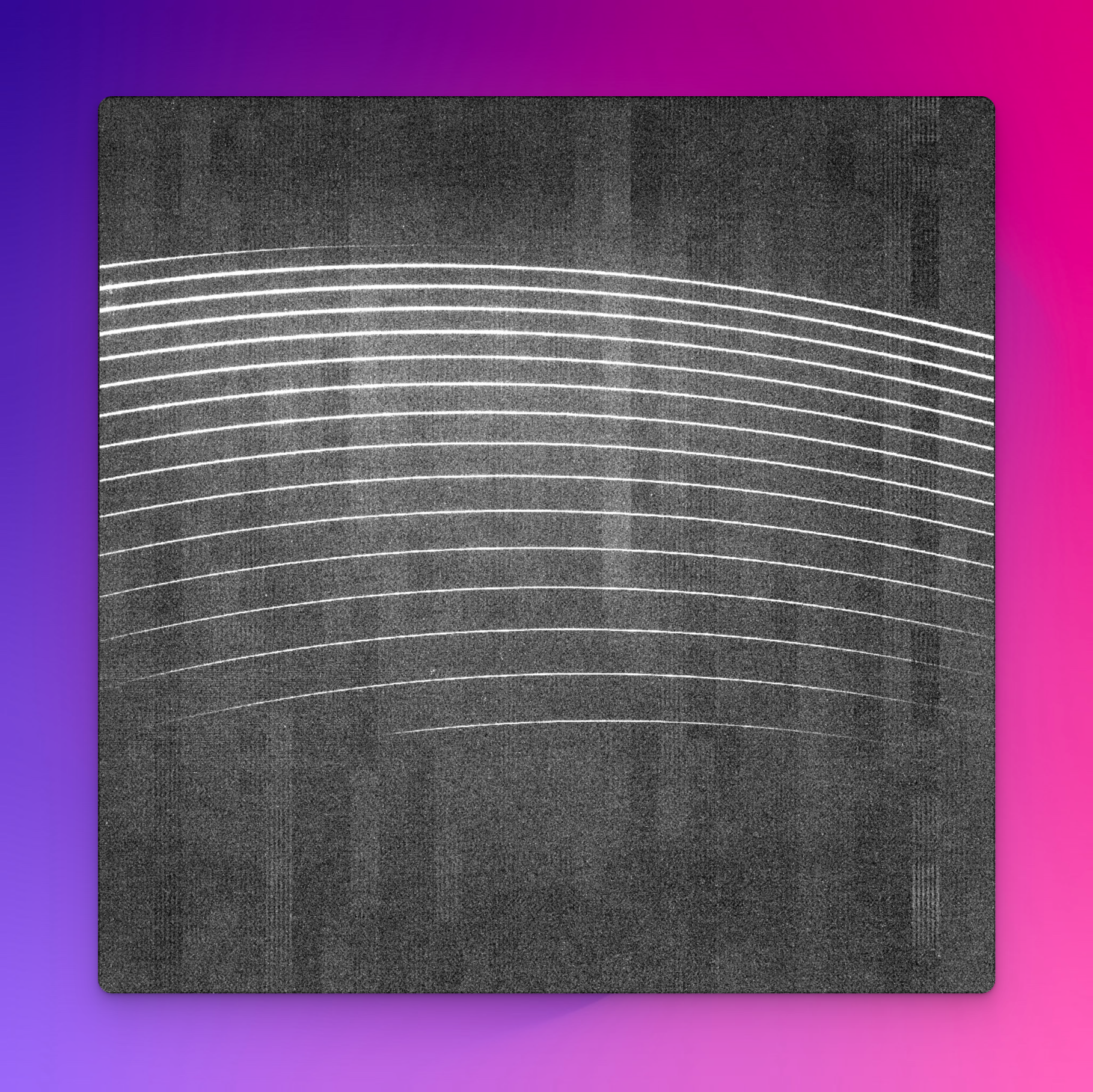
Fig. 61 A 15-second QTH flat-lamp exposure through a pinhole mask onto the SOXS NIR detector.

From a spectral format table (specific to the arm in question), the minimum and maximum wavelength values for each order are known. The first guess dispersion map generated by soxs_disp_solution generates an array of pixel locations along the centre of each order between these wavelength limits.

Centred on each pixel position, an N-pixel long (slice-length recipe parameter), M-pixel wide (slice-width recipe parameter) image slice is taken in the cross-dispersion direction. Each slice is collapsed to 1 pixel in width by taking the median pixel value at each location along the length of the slice. A 1D gaussian is fitted to the flux in each slice, and if a peak is registered with more than a peak-sigma-limit sigma significance, the pixel-position is stored (see Fig. 62 and Fig. 63).

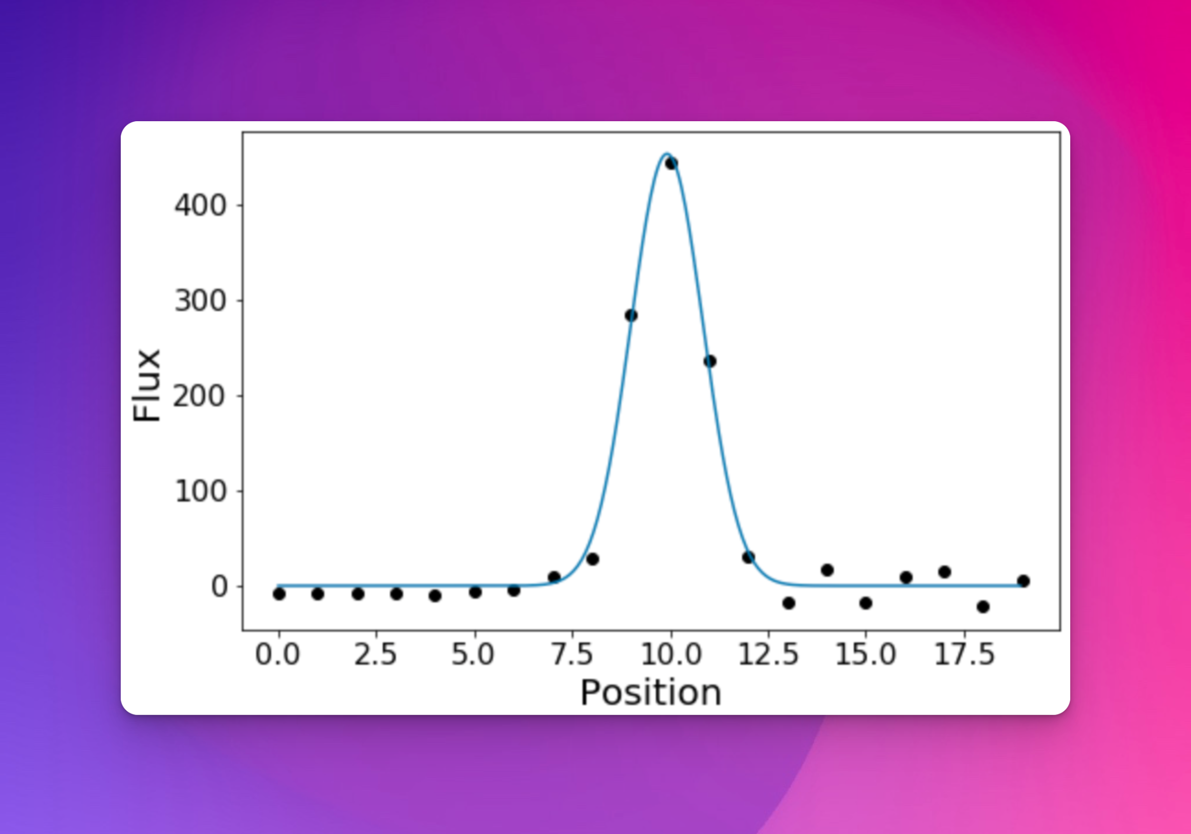
Fig. 62 An attempt is made to fit a Gaussian to the flux in each slice. The pixel position is stored if a peak is registered with more than a peak-sigma-limit sigma significance.

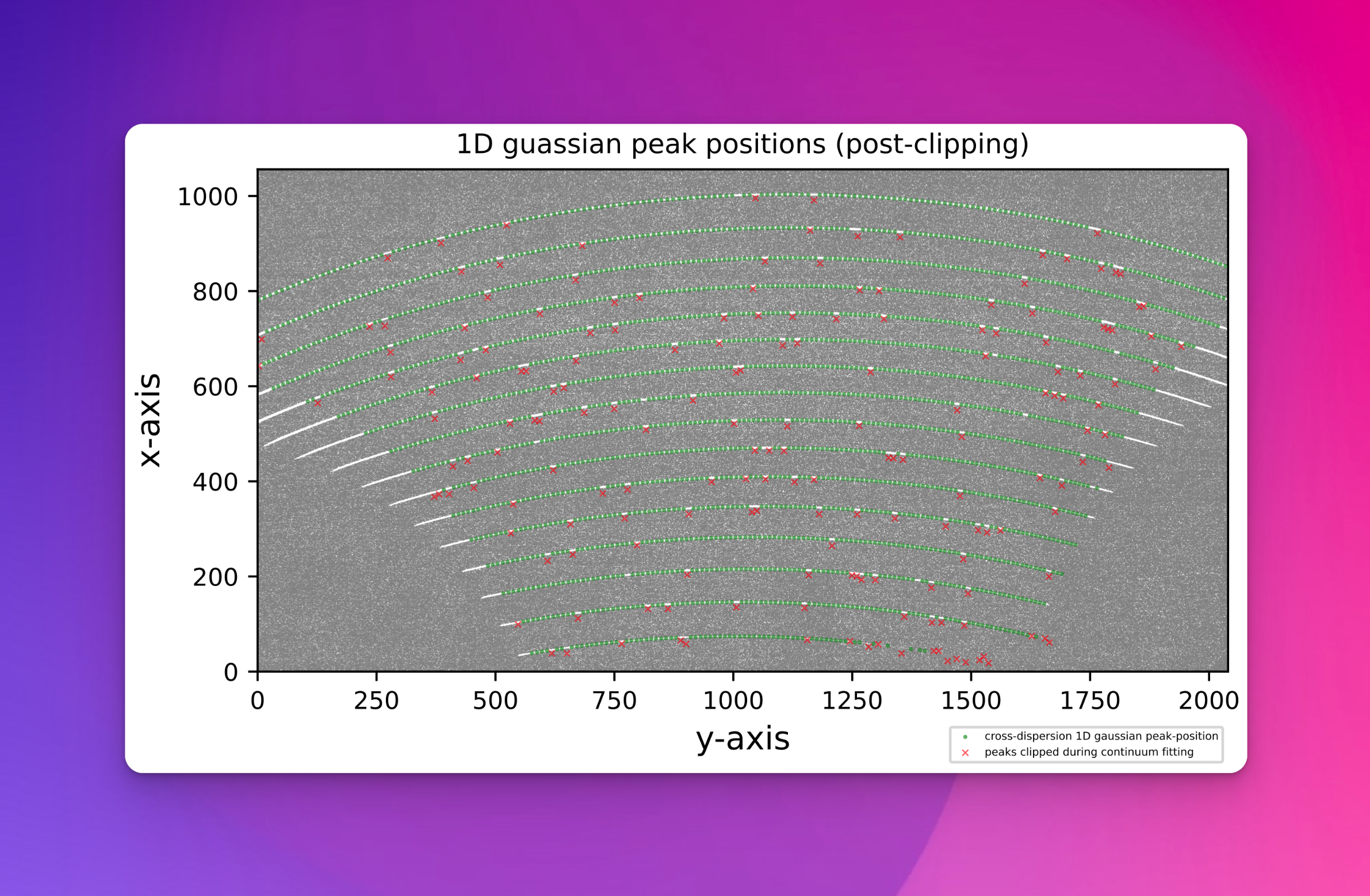
Fig. 63 The green circles represent the location on the cross-dispersion slice where a flux peak was detected. The red crosses show the centre of the slices where a peak failed to be detected.

Finally, the entire set of Gaussian peak pixel positions is iteratively fitted with a polynomial:

\[ X = \sum\limits_{ij} c_{ij} \times n^i \times Y^j \]

where \(X\) and \(Y\) are the pixel positions and \(n\) is the echelle order number. \(i\) and \(j\) are the polynomial degree orders for the echelle order (order-deg) and \(Y\) pixel position (disp-axis-deg) respectively. \(c_{ij}\) are the polynomial coefficients to be fitted. The polynomial is iteratively fitted while sigma-clipping pixel-positions with outlying residuals. As this is a global fit to the source trace across all orders, even if the source is very faint in a few orders, it still has a good chance of fitting a trace. The final results are stored in an order location table.

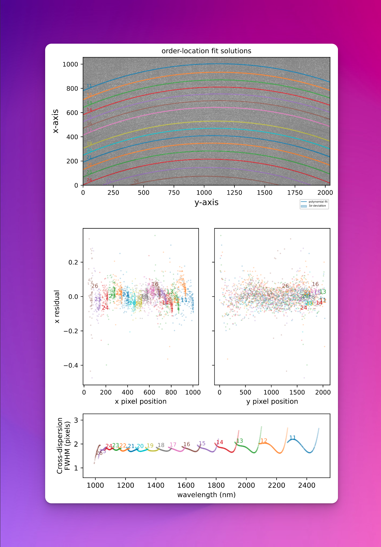
Fig. 64 The top panel show the global polynomial fitted to the detected source trace with the different colours representing individual echelle orders. The middle panels show the fit residuals in the X and Y axes. The bottom panel shows the FWHM of the trace fits (in pixels) with respect to echelle order and wavelength.

Utility API

class detect_continuum(log, traceFrame, dispersion_map, settings=False, recipeSettings=False, recipeName=False, qcTable=False, productsTable=False, sofName=False, binx=1, biny=1, lampTag=False, locationSetIndex=False, orderPixelTable=False, startNightDate='', debug=False)

Bases: soxspipe.commonutils.detect_continuum._base_detect

find and fit the continuum trace across all echelle orders with low-order polynomials.

Key Arguments:

• log – logger

• traceFrame – calibrated frame containing a source trace (CCDObject)

• dispersion_map – path to dispersion map file containing polynomial fits of the dispersion solution for the frame

• settings – the settings dictionary

• recipeSettings – the recipe specific settings

• recipeName – the recipe name as given in the settings dictionary

• qcTable – the data frame to collect measured QC metrics

• productsTable – the data frame to collect output products

• sofName —- name of the originating SOF file

• binx – binning in x-axis

• biny – binning in y-axis

• lampTag – add this tag to the end of the product filename. Default False

• locationSetIndex – the index of the AB cycle locations (nodding mode only). Default False

• orderPixelTable – this is used for tuning the pipeline. Default False

• startNightDate – YYYY-MM-DD date of the observation night. Default “”

• debug – if True then extra debugging information is printed. Default False

Usage:

To use the detect_continuum object, use the following:

from soxspipe.commonutils import detect_continuum
detector = detect_continuum(
    log=log,
    traceFrame=traceFrame,
    dispersion_map=dispersion_map,
    settings=settings,
    recipeName="soxs-order-centres"
)
order_table_path = detector.get()

Initialization

calculate_residuals(orderPixelTable, coeff, axisACol, axisBCol, orderCol=False, writeQCs=False)

create_pixel_arrays()

create a pixel array for the approximate centre of each order

Return:

• orderPixelTable – a data-frame containing lines and associated pixel locations

• dmBinx – the dispersion map binning in x

• dmBiny – the dispersion map binning in y

fit_1d_gaussian_to_slices(orderPixelTable, sliceLength, medianStddev=False)

Optimized version of Gaussian fitting to slices

fit_global_polynomial(pixelList, axisACol='cont_x', axisBCol='cont_y', orderCol='order', exponentsIncluded=False, writeQCs=False)

fit_order_polynomial(pixelList, order, axisBDeg, axisACol, axisBCol, exponentsIncluded=False)

get()

return the order centre table filepath

Return:

• order_table_path – file path to the order centre table giving polynomial coeffs to each order fit

plot_results(orderPixelTable, orderPolyTable, clippedData)

generate a plot of the polynomial fits and residuals

Key Arguments:

• orderPixelTable – the pixel table with residuals of fits

• orderPolyTable – data-frame of order-location polynomial coeff

• clippedData – the sigma-clipped data

Return:

• filePath – path to the plot pdf

• orderMetaTable – dataframe of useful order fit metadata

sample_trace()

take many cross-dispersion samples across each order to try and find an object trace

Return:

• orderPixelTable – the detector locations at which a trace was found

write_order_table_to_file(frame, orderPolyTable, orderMetaTable)