create_dispersion_map ∞
The create_dispersion_map utility is used to search for arc-lines in the single/multi-pinhole arc-lamp frames and then iteratively fit a global polynomial dispersion solution (and spatial-solution in the case of multi-pinhole frame) with the observed line-positions. It is used by both the soxs_disp_solution) and soxs_spatial_solution) solution recipes.
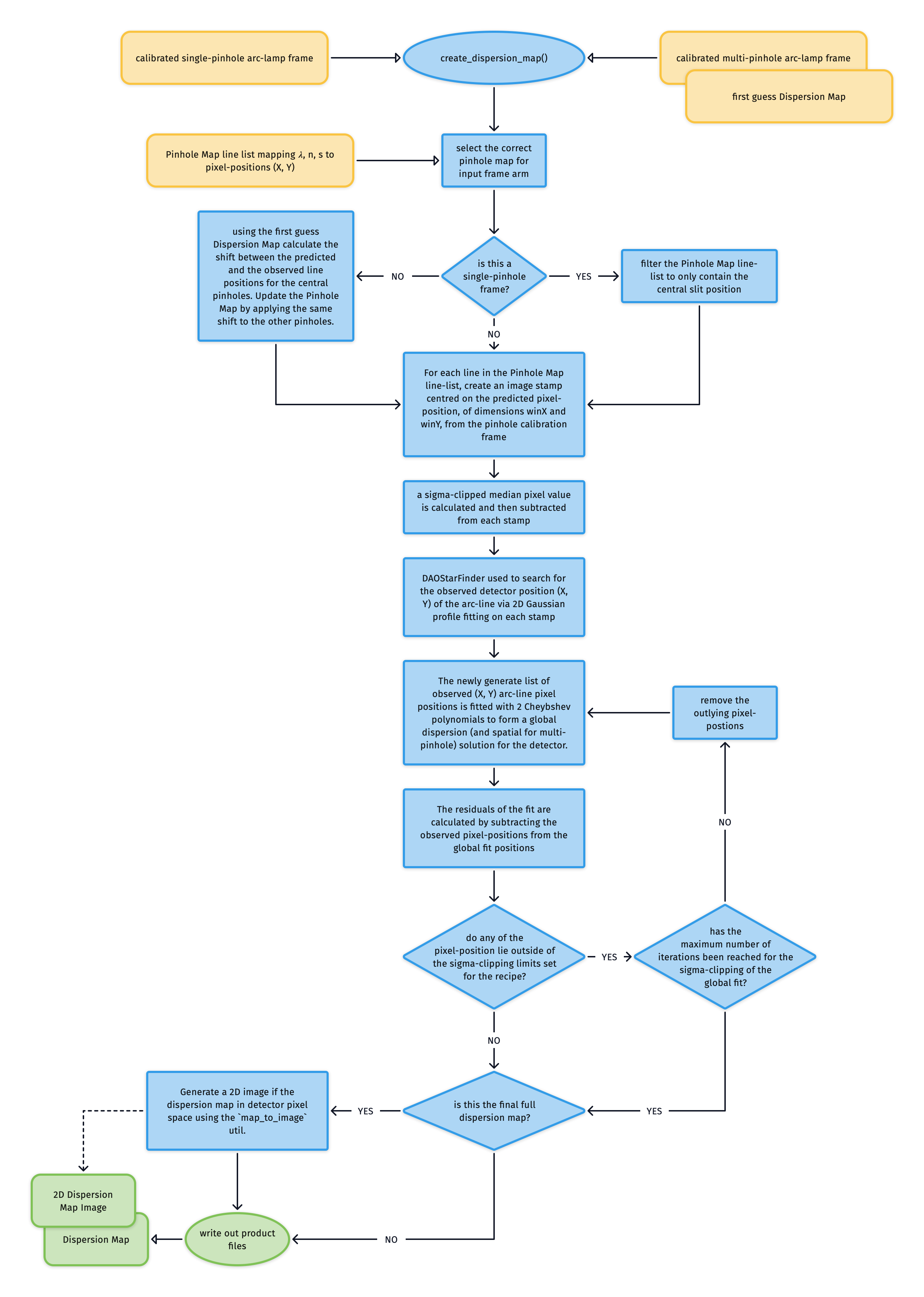
In the static calibration suite we have Pinhole Maps listing the wavelength \(\lambda\), order number \(n\) and slit position \(s\) of the spectral lines alongside a first approximation of their (\(X, Y\)) pixel-positions on the detector.
If the input frame is a single-pinhole frame, we can filter the Pinhole Map to contain just the central pinhole positions. If however input is the multi-pinhole frame then we use the first guess Dispersion Map (created with soxs_disp_solution) to calculate the shift between the predicted and the observed line positions for the central pinholes. We then update the Pinhole Map by applying the same shift to the other pinholes.
For each line in the Pinhole Map line-list:
an image stamp centred on the predicted pixel-position (\(X_o, Y_o\)), of dimensions winX and winY, is generated from the pinhole calibration frame
a sigma-clipped median pixel value is calculated and then subtracted from each stamp
DAOStarFinder is employed to search for the observed detector position (\(X, Y\)) of the arc-line via 2D Gaussian profile fitting on the stamp
We now have a list of arc-line wavelengths and their observed pixel-positions and the order they were detected in. These values are used to iteratively fit two polynomials that describe the global dispersion solution for the detector. In the case of the single-pinhole frames these are:
where \(\lambda\) is wavelength and \(n\) is the echelle order number.
In the case of the multi-pinhole we also have the slit position \(s\) and so adding a spatial solution to the dispersion solution:
Upon each iteration the residuals between the fits and the measured pixel-positions are calculated and sigma-clipping is employed to eliminate measurements that stray to far from the fit. Once the maximum number of iterations is reach, or all outlying lines have been clipped, the coefficients of the polynomials are written to a Dispersion Map file.
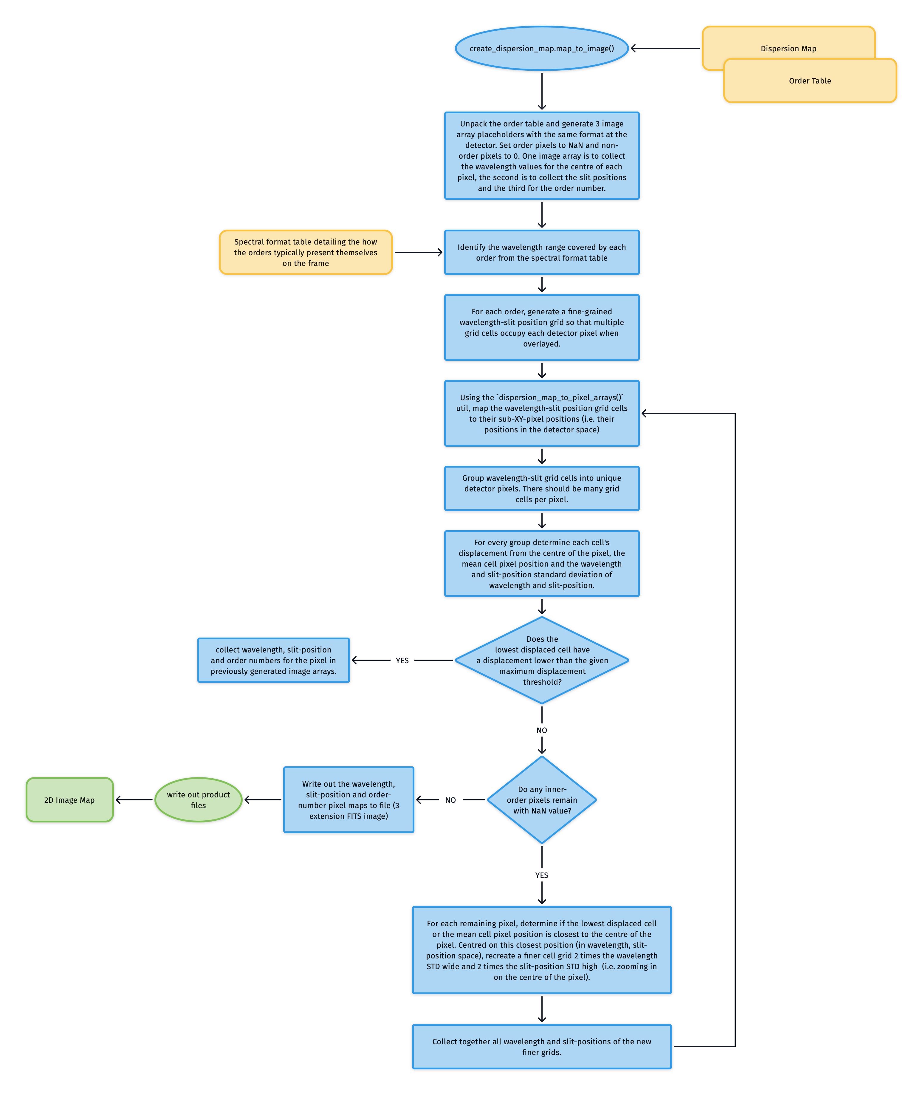
2D Image Map ∞

The Dispersion Map is used to generate a triple extension FITS file with each extension image exactly matching the dimensions of the detector. The first extension contains the wavelength value at the centre of each pixel location, the second the slit-position and the third the order number. The solutions for these images are iteratively converged on in a brute force manner (see workflow diagram below). These image maps are used in sky-background subtraction and object extraction utilities.
-
class
create_dispersion_map(log, settings, recipeSettings, pinholeFrame, firstGuessMap=False, orderTable=False, qcTable=False, productsTable=False, sofName=False, create2DMap=True)[source] ∞ detect arc-lines on a pinhole frame to generate a dispersion solution
- Key Arguments:
log– loggersettings– the settings dictionaryrecipeSettings– the recipe specific settingspinholeFrame– the calibrated pinhole frame (single or multi)firstGuessMap– the first guess dispersion map from thesoxs_disp_solutionrecipe (needed insoxs_spat_solutionrecipe). Default False.orderTable– the order geometry tableqcTable– the data frame to collect measured QC metricsproductsTable– the data frame to collect output productssofName– name of the originating SOF filecreate2DMap– create the 2D image map of wavelength, slit-position and order from disp solution.
Usage:
from soxspipe.commonutils import create_dispersion_map
mapPath, mapImagePath, res_plots, qcTable, productsTable = create_dispersion_map(
    log=log,
    settings=settings,
    pinholeFrame=frame,
    firstGuessMap=False,
    qcTable=self.qc,
    productsTable=self.products
).get()
-
get()[source] ∞ generate the dispersion map
- Return:
mapPath– path to the file containing the coefficients of the x,y polynomials of the global dispersion map fit
-
get_predicted_line_list()[source] ∞ lift the predicted line list from the static calibrations
- Return:
orderPixelTable– a panda’s data-frame containing wavelength,order,slit_index,slit_position,detector_x,detector_y
-
detect_pinhole_arc_line(predictedLine, iraf=True)[source] ∞ detect the observed position of an arc-line given the predicted pixel positions
- Key Arguments:
predictedLine– single predicted line coordinates from predicted line-listiraf– use IRAF star finder to generate a FWHM
- Return:
predictedLine– the line with the observed pixel coordinates appended (if detected, otherwise nan)
-
write_map_to_file(xcoeff, ycoeff, orderDeg, wavelengthDeg, slitDeg)[source] ∞ write out the fitted polynomial solution coefficients to file
- Key Arguments:
xcoeff– the x-coefficientsycoeff– the y-coefficientsorderDeg– degree of the order fittingwavelengthDeg– degree of wavelength fittingslitDeg– degree of the slit fitting (False for single pinhole)
- Return:
disp_map_path– path to the saved file
-
calculate_residuals(orderPixelTable, xcoeff, ycoeff, orderDeg, wavelengthDeg, slitDeg, writeQCs=False, pixelRange=False)[source] ∞ calculate residuals of the polynomial fits against the observed line positions
Key Arguments:
orderPixelTable– the predicted line list as a data framexcoeff– the x-coefficientsycoeff– the y-coefficientsorderDeg– degree of the order fittingwavelengthDeg– degree of wavelength fittingslitDeg– degree of the slit fitting (False for single pinhole)writeQCs– write the QCs to dataframe? Default FalsepixelRange– return centre pixel and +- 2nm from the centre pixel (to measure the pixel scale)
- Return:
residuals– combined x-y residualsmean– the mean of the combine residualsstd– the stdev of the combine residualsmedian– the median of the combine residuals
-
fit_polynomials(orderPixelTable, wavelengthDeg, orderDeg, slitDeg, missingLines=False)[source] ∞ iteratively fit the dispersion map polynomials to the data, clipping residuals with each iteration
- Key Arguments:
orderPixelTable– data frame containing order, wavelengths, slit positions and observed pixel positionswavelengthDeg– degree of wavelength fittingorderDeg– degree of the order fittingslitDeg– degree of the slit fitting (0 for single pinhole)missingLines– lines not detected on the image
- Return:
xcoeff– the x-coefficients post clippingycoeff– the y-coefficients post clippinggoodLinesTable– the fitted line-list with metricsclippedLinesTable– the lines that were sigma-clipped during polynomial fitting
-
create_placeholder_images(order=False, plot=False, reverse=False)[source] ∞ create CCDData objects as placeholders to host the 2D images of the wavelength and spatial solutions from dispersion solution map
- Key Arguments:
order– specific order to generate the placeholder pixels for. Inner-order pixels set to NaN, else set to 0. Default False (generate all orders)plot– generate plots of placeholder images (for debugging). Default False.reverse– Inner-order pixels set to 0, else set to NaN (reverse of default output).
- Return:
slitMap– placeholder image to add pixel slit positions towlMap– placeholder image to add pixel wavelength values to
Usage:
slitMap, wlMap, orderMap = self._create_placeholder_images(order=order)
-
map_to_image(dispersionMapPath)[source] ∞ convert the dispersion map to images in the detector format showing pixel wavelength values and slit positions
- Key Arguments:
dispersionMapPath– path to the full dispersion map to convert to images
- Return:
dispersion_image_filePath– path to the FITS image with an extension for wavelength values and another for slit positions
Usage:
mapImagePath = self.map_to_image(dispersionMapPath=mapPath)
-
order_to_image(orderInfo)[source] ∞ convert a single order in the dispersion map to wavelength and slit position images
- Key Arguments:
orderInfo– tuple containing the order number to generate the images for, the minimum wavelength to consider (from format table) and maximum wavelength to consider (from format table).
- Return:
slitMap– the slit map with order values filledwlMap– the wavelengths map with order values filled
Usage:
slitMap, wlMap = self.order_to_image(order=order,minWl=minWl, maxWl=maxWl)
-
convert_and_fit(order, bigWlArray, bigSlitArray, slitMap, wlMap, iteration, plots=False)[source] ∞ convert wavelength and slit position grids to pixels
- Key Arguments:
order– the order being consideredbigWlArray– 1D array of all wavelengths to be convertedbigSlitArray– 1D array of all split-positions to be converted (same length asbigWlArray)slitMap– place-holder image hosting fitted pixel slit-position valueswlMap– place-holder image hosting fitted pixel wavelength valuesiteration– the iteration index (used for CL reporting)plots– show plot of the slit-map
- Return:
orderPixelTable– dataframe containing unfitted pixel inforemainingCount– number of remaining pixels in orderTable
Usage:
orderPixelTable = self.convert_and_fit(
        order=order, bigWlArray=bigWlArray, bigSlitArray=bigSlitArray, slitMap=slitMap, wlMap=wlMap)
-
create_new_static_line_list(dispersionMapPath)[source] ∞ using a first pass dispersion solution, use a line atlas to generate a more accurate and more complete static line list
Key Arguments:
- `dispersionMapPath` -- path to the first pass dispersion solution
Return:
- `newPredictedLineList` -- a new predicted line list (to replace the static calibration line-list)