Spectroscopic Data Reduction Cascade
One of the most challenging problems the SOXS pipeline has to overcome is the curvature of the NIR spectral orders. Also, although the UVB-VIS orders should be aligned linearly along the CCD columns, the observed emission lines will not be perpendicular to the source trace but exhibit a slight tilt that must also be accounted for.
Here is a brief overview of the individual reduction steps performed by the pipeline on the spectroscopic data (also shown in Fig. 31):
Individual object frames are prepared by trimming and adding bad-pixel and error map extensions.
The bias current is removed, either via subtraction of a master bias frame (stare mode) or via the A-B and B-A cycle subtractions (nodding and offset modes).
Any dark current is removed, either via the subtraction of a master dark frame (NIR only) or via the A-B and B-A cycle subtractions (nodding and offset modes).
Frames are divided by a master-flat frame.
The inter-order background (mainly due to scattered light registering on the detector) is fitted and removed from the frames.
The signal from the sky background is either modelled from the object frame and removed (stare mode) or removed during A-B and B-A cycle subtractions (nodding and offset modes).
The object signal is traced and optimally extracted (using the object’s profile modelled according to the prescription of Horne [Hor86]) from individual orders in the original detector pixel space. Unlike other pipelines, we do not rectify the curved orders onto a straight grid before extraction, as this process is known to increase/add a correlated noise component to the data. An additional boxcar extraction is performed on the object trace.
The individual order extractions are merged into a single spectrum (UV-VIS 350-850nm, NIR 800-2000 nm).
The identical processes above are applied to a flux standard star, taken close in time to the science object, and the order-merged extraction of this standard star is compared against its catalogued calibrated spectrum to determine the instrument’s response function.
The object spectrum is flux-calibrated with the response curve calculated in the previous step.
Since the arc-lamp frames used to determine the dispersion solution are taken during the afternoon, a check of the wavelength calibration is made using the position of sky emission lines. Any systematic offset observed in the extracted spectra is corrected for. (YET TO BE IMPLEMENTED. This will work for the NIR but could be extended to UVVIS, although it should be clarified if the correction is feasible due to the lower number of lines from the sky available in these regions).
The ESO package MOLECFIT is run on the flux and wavelength-calibrated 1D spectra to remove the telluric absorption (YET TO BE IMPLEMENTED).
In addition to the 1D reduced and calibrated spectra, a flux and wavelength-calibrated, order-merged 2D image is produced. This will allow users to extract their 1D spectrum.
Finally, using the wavelength overlap (~50nm) between the arms to cross-calibrate flux, the order-merged 1D extractions from the individual arms are merged to form a single object extraction.
End-to-end error propagation is carried out throughout the cascade to produce the final variance spectrum, which contains all noise sources. For more details on the individual reduction stages, see the recipes section.
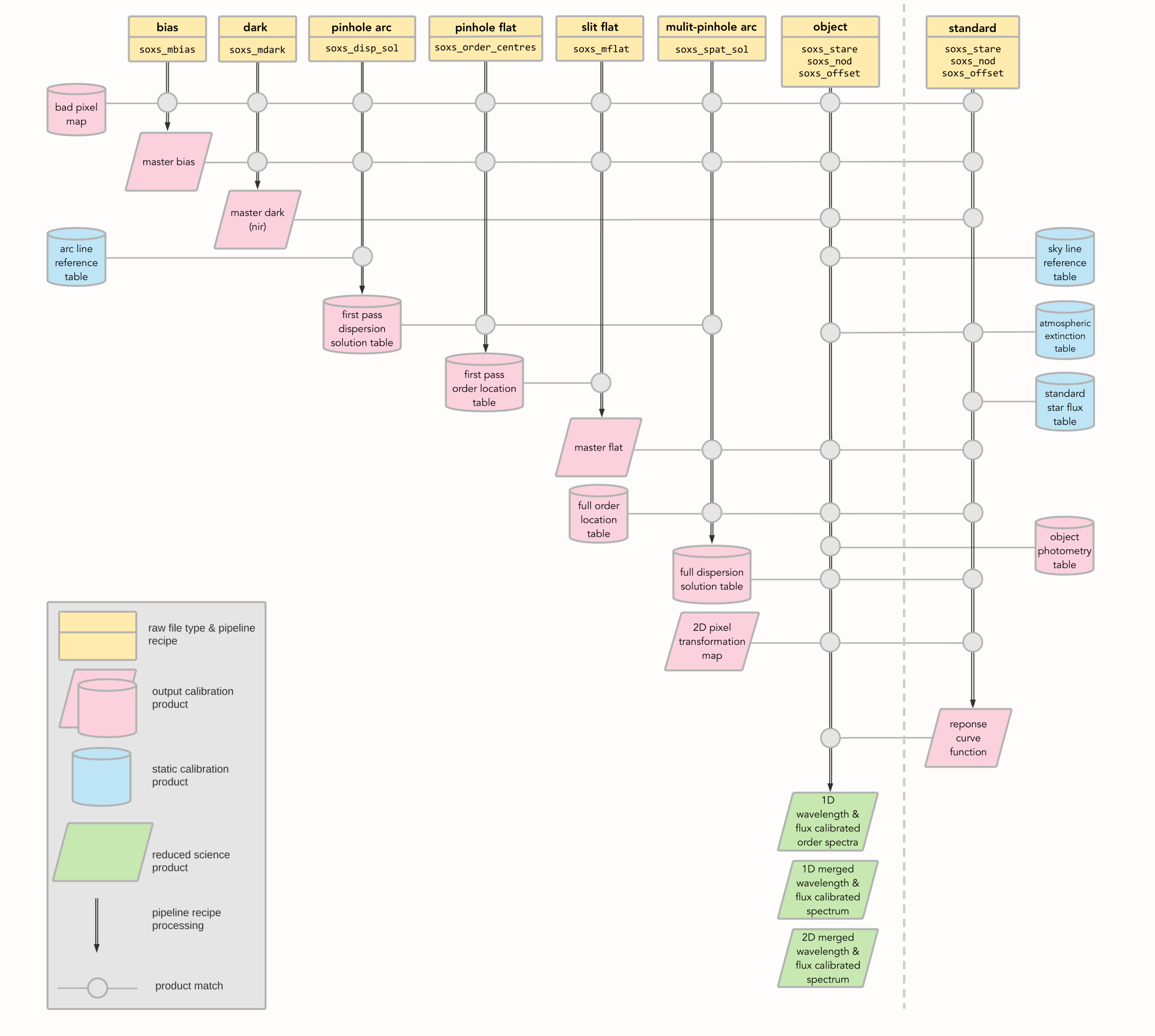
Fig. 31 The SOXS spectroscopic data reduction cascade. The input data, calibration products required and the output frames are shown for each pipeline recipe implemented in the pipeline. Vertical lines in the map depict a raw data frame, the specific recipe to be applied to that frame and the data product(s) output by that recipe. Horizontal lines show how subsequent pipeline recipes use those output data products. Time loosely proceeds from left to right (recipe order) and top to bottom (recipe processing steps) on the map. To the right of the grey dashed line are input calibration products generated from a separate pipeline processing cascade.
Spectroscopic Data
Daily Calibration Data
Bias frames (UV-VIS only)
Dark frames (NIR only)
Through-slit flat field frames (UV-VIS/NIR)
Single pinhole arc-lamp frames
Single pinhole flat-field frame
Multiple pinhole arc-lamp frames
Spectrophotmetric standard star observations
Regular linearity test data
Static Calibration Data
Reference bad pixel map
Line reference table to wavelength calibrate spectra (wavelength solution is in air)
Standard star flux table
Atmospheric extinction table
Sky Lines reference table
Intermediate Data Products
Master bias frame
Master dark frame
Master flat-frame
Order location table
Dispersion solution table
Instrument response function
Output Data Products
Product |
Description |
|---|---|
1D Source Spectra |
1D spectra in FITS binary table format, one for each arm. Each FITS spectrum file will contain four extensions: 1. Wavelength- and flux-calibrated spectra with absolute flux correction via scaling to acquisition image source photometry, 2. an additional spectrum with correction for telluric absorption via MOLECFIT, 3. the variance array and 4. the sky-background spectra. |
1D Merged Source Spectrum |
1D UV-VIS & NIR merged spectrum in FITS binary table format with PDF visualisation. This spectrum will be rebinned to a common pixel scale for each arm. This spectrum file will also have the same four extensions described above. |
2D Source Spectra |
A 2D FITS image for each spectral arm containing wavelength and flux calibrated spectra (no other corrections applied) allows users to perform source extraction with their tool of choice. Note that rectifying the curved orders in the NIR introduces a source of correlated noise not present in extractions performed on the un-straightened orders as done by the pipeline. |