soxs_spatial_solution

The soxs_spatial_solution recipe enhances the wavelength solution achieved with soxs_disp_solution by expanding the solution into the spatial dimension (along the slit). The resulting 2-dimensional solution accounts for any tilt in the spectral lines relative to the cross-dispersion axis. The recipe is similar in logic to soxs_disp_solution, but now samples arc lines along the slit in the cross-dispersion direction using a multi-pinhole slit mask.

Input

Table 71 Input files for the soxs_spatial_solution recipe. The files are typically passed to the soxs_spatial_solution recipe via a set-of-file (sof) file listing one file per line.

Data Type	Content	Related OB
FITS Image	Arc Lamp through multi-pinhole mask	SOXS_slt_cal_VISArcsMultiplePinhole, SOXS_slt_cal_NIRArcsMultiplePinhole
FITS Image	Master Dark Frame (VIS only, optional)	-
FITS Image	Master Bias Frame (VIS only)	-
FITS Image	Master Flat Frame (optional)	-
FITS Image	Dark frame (Lamp-Off) of equal exposure length as multi-pinhole frame (Lamp-On) (NIR only)	SOXS_slt_cal_NIRArcsMultiplePinhole
FITS Table	First-guess Dispersion map table

Table 72 Ancillary (static) files required by the soxs_spatial_solution recipe. These files are packaged with and shipped with the code.

Data Type	Content
FITS images	Default bad-pixel map
FITS Binary Table	A spectral format table for the detector, giving the minimum and maximum wavelengths covered by each spectral order.
FITS Binary Table	An arc-lamp line list. This table gives the predicted x, y pixel position that each arc line is expected to appear near for each spectral order and pinhole in the multi-pinhole mask.

Parameters

Table 73 The soxs_spatial_solution recipe parameters.

Parameter	Description	Type	Entry Point	Related Util
use_flat	divide image by master flat frame	bool	settings	-
subtract_background	fit and subtract the intra-order background light	bool	settings	subtract_background
pixel_window_size	the size of the square window used to search for an arc-lamp emission line, centred on the predicted pixel position of the line	int	settings	create_dispersion_map
pinhole_detection_thres_sigma	minimum significance required for arc-line to be considered ‘detected’	float	settings	create_dispersion_map
order_deg	degree of echelle order number component of global polynomial fit to the dispersion solution [x, y]	int/list	settings file or command-line	create_dispersion_map
wavelength_deg	degree of wavelength component of global polynomial fit to the dispersion solution [x, y]	int/list	settings file or command-line	create_dispersion_map
slit_deg	degree of slit position component of global polynomial fit to the dispersion solution [x, y]	int/list	settings file or command-line	create_dispersion_map
poly_clipping_iteration_limit	number of sigma-clipping iterations to perform before settings on a polynomial fit for the dispersion solution	int	settings	create_dispersion_map
poly_fitting_residual_clipping_sigma	sigma clipping limit when fitting global polynomial to the dispersion solution	float	settings	create_dispersion_map
poly_clipping_pinhole_sets	clipping performed on multi-pinhole sets (true) or individual pinholes (false)	bool	settings	create_dispersion_map
map_to_image_displacement_threshold	maximum distance allowed from the pixel centre when calculating wavelength, order and slit-position for 2d disp-sol image	float	settings	create_dispersion_map
mph_line_set_min	full multi-pinholes sets (same arc line) with fewer than mph_line_set_min lines detected get clipped	int	settings	create_dispersion_map
background_subtraction: bspline_deg	degree of bsplines used to fit the inter-order background (if subtract_background == True)	int	settings file	subtract_background
background_subtraction: gaussian_blur_sigma	Standard deviation of Gaussian kernel used to smooth background image (if subtract_background == True)	int	settings file	subtract_background

Method

The algorithm used in the soxs_spatial_solution recipe is shown in Fig. 47.

Having prepared the multi-pinhole frame, the bias and dark signatures are removed, and the frame is divided through by the master flat frame. The calibrated frame and the first-guess dispersion map are passed to the create_dispersion_map utility, arc-lines from a static line-list are detected and fitted to produce a 2D dispersion solution covering both the spectral and spatial dimensions. Note that saturated arc-lines are either absent from the input line-list file or get clipped during the fitting process and so are not included in the final dispersion solution fitting.

A three-extension FITS image with the same format as the detector is created using the complete dispersion solution. The first extension contains the wavelength values for each pixel, the second the slit positions, and the third the echelle order number.

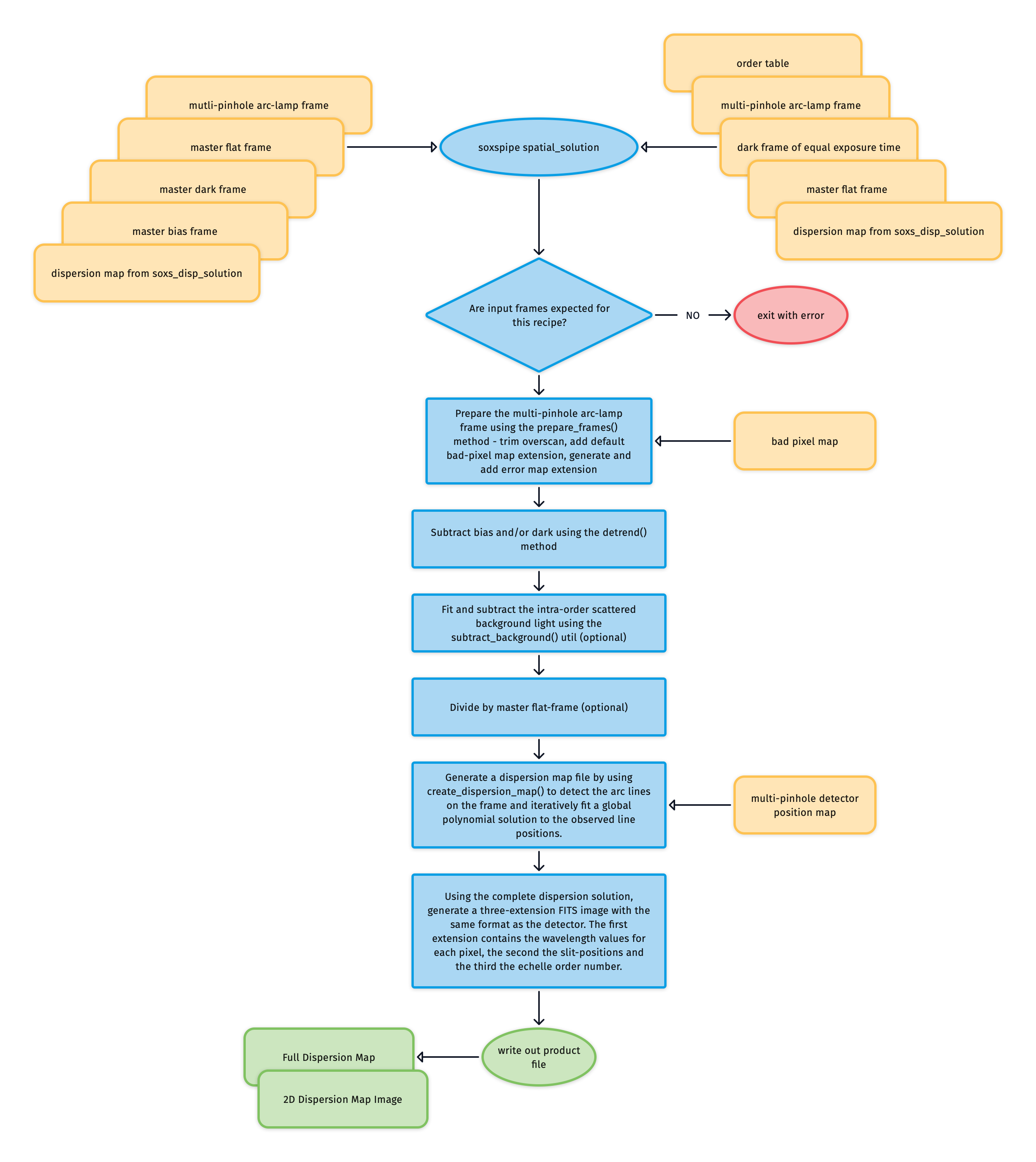
Fig. 47 The soxs_spatial_solution recipe algorithm. At the top of the diagram, NIR input data is found on the right and VIS on the left.

Output

Table 74 Output files for the soxs_spatial_solution recipe and their respective ESO PRO keywords.

Label	Content	Data Type	PRO CATG	PRO TYPE	PRO TECH
SPAT SOL	Full dispersion-spatial solution	FITS	DISP_TAB_<ARM>	REDUCED	ECHELLE,MULTI-PINHOLE
2D MAP	2D detector map of wavelength, slit position and order	FITS	DISP_IMAGE_<ARM>	REDUCED	ECHELLE,MULTI-PINHOLE
BKGROUND	Fitted intra-order image background	PDF	-	-	-
DISP MAP LINES	Dispersion solution fitted lines	FITS	-	-	-
DISP MAP LINES MISSING	Undetected arc lines	FITS	-	-	-
DISP MAP RES	Dispersion solution QC plots	PDF	-	-	-

QC Metrics

Table 75 Quality Control metrics calculated in the soxs_spatial_solution recipe.

Label	Description	Unit	Acceptable Range
DETLINES CLIP NUM	Total number of detected lines clipped during solution fitting	lines	-
DETLINES NUM	Number of lines detected in single pinhole frame	lines	-
DETLINES FRAC	Proportion of input line-list lines detected on single pinhole frame		VIS: [0.95,1.0]
DETLINES TOT	Total number of line in single line-list	lines	-
GOODLINES FRAC	Proportion of good, unclipped lines in single pinhole frame	lines	VIS: [0.55,1.0] NIR: [0.4,1.0]
PINHOLE COUNT MIN	The minimum number of pinholes found across all orders (should be 9)	pinholes	VIS: 9, NIR: 9
X RES MAX	Maximum residual in fitting of pinholes along x-axis (global)	pixels	-
X RES MIN	Minimum residual in fitting of pinholes along x-axis (global)	pixels	-
X RES MEDIAN	Median of absolute residuals in fitting of pinholes along x-axis (global)	pixels	-
X RES SD	Std-dev of residuals in fitting of pinholes along x-axis (global)	pixels	VIS: [0,0.25], NIR: [0,0.42]
Y RES MAX	Maximum residual in fitting of pinholes along y-axis (global)	pixels	-
Y RES MIN	Minimum residual in fitting of pinholes along y-axis (global)	pixels	-
Y RES MEDIAN	Median of absolute residuals in fitting of pinholes along y-axis (global)	pixels	-
Y RES SD	Std-dev of residuals in fitting of pinholes along y-axis (global)	pixels	VIS: [0,0.48], NIR: [0,0.12]
XY RES MAX	Maximum residual in fitting of pinholes (global)	pixels	-
XY RES MIN	Minimum residual in fitting of pinholes (global)	pixels	-
XY RES MEDIAN	Median residual in fitting of pinholes (global)	pixels	VIS: [0,0.7], NIR: [0,0.3]
XY RES SD	Std-dev of residuals in fitting of pinholes (global)	pixels	VIS: [0,0.5], NIR: [0,0.4]
X DIFF MEDIAN	Median difference between observed and predicted pinhole detector locations along the x-axis (global)	pixels	-
X DIFF SD	Standard deviation in difference between observed and predicted pinhole detector locations along the x-axis (global)	pixels	-
Y DIFF MEDIAN	SMedian difference between observed and predicted pinhole detector locations along the y-axis (global)	pixels	-
Y DIFF SD	Standard deviation in difference between observed and predicted pinhole detector locations along the y-axis (global)	pixels	-
XY DIFF MEDIAN	Median difference between observed and predicted pinhole detector locations (global)	pixels	-
XY DIFF SD	Standard deviation of difference between observed and predicted pinhole detector locations (global)	pixels	-
FWHM PIN MEDIAN	Median FWHM of detected lines in pinhole frames (global)	pixels	VIS: [1.60,1.72], NIR: [1.55,1.85]
FWHM PIN SD	Standard deviation in FWHM of detected lines in pinhole frames (global)	pixels	VIS: [0.0,0.16], NIR: [0.0,0.145]
R PIN MEDIAN	Median spectral resolution measured from detected lines in pinhole frames (global)		-
X RES MAX O<N>	Maximum residual in fitting of pinholes along x-axis (order N)	pixels	-
X RES MIN O<N>	Minimum residual in fitting of pinholes along x-axis (order N)	pixels	-
X RES MEDIAN O<N>	Median of absolute residuals in fitting of pinholes along x-axis (order N)	pixels	-
X RES SD O<N>	Std-dev of residuals in fitting of pinholes along x-axis (order N)	pixels	-
Y RES MAX O<N>	Maximum residual in fitting of pinholes along y-axis (order N)	pixels	-
Y RES MIN O<N>	Minimum residual in fitting of pinholes along y-axis (order N)	pixels	-
Y RES MEDIAN O<N>	Median of absolute residuals in fitting of pinholes along y-axis (order N)	pixels	-
Y RES SD O<N>	Std-dev of residuals in fitting of pinholes along y-axis (order N)	pixels	-
XY RES MAX O<N>	Maximum residual in fitting of pinholes (order N)	pixels	-
XY RES MIN O<N>	Minimum residual in fitting of pinholes (order N)	pixels	-
XY RES SD O<N>	Std-dev of residuals in fitting of pinholes along (order N)	pixels	-
X DIFF MEDIAN O<N>	Median difference between observed and predicted pinhole detector locations along the x-axis (order N)	pixels	-
X DIFF SD O<N>	Standard deviation in difference between observed and predicted pinhole detector locations along the x-axis (order N)	pixels	-
Y DIFF MEDIAN O<N>	SMedian difference between observed and predicted pinhole detector locations along the y-axis (order N)	pixels	-
Y DIFF SD O<N>	Standard deviation in difference between observed and predicted pinhole detector locations along the y-axis (order N)	pixels	-
XY DIFF MEDIAN O<N>	Median difference between observed and predicted pinhole detector locations (order N)	pixels	-
FWHM PIN MEDIAN O<N>	Median FWHM of detected lines in pinhole frames (order N)	pixels	-
FWHM PIN SD O<N>	Standard-deviation in FWHM of detected lines in pinhole frames (order N)	pixels	-
R PIN MEDIAN O<N>	Median spectral resolution measured from detected lines in pinhole frames (order N)		-

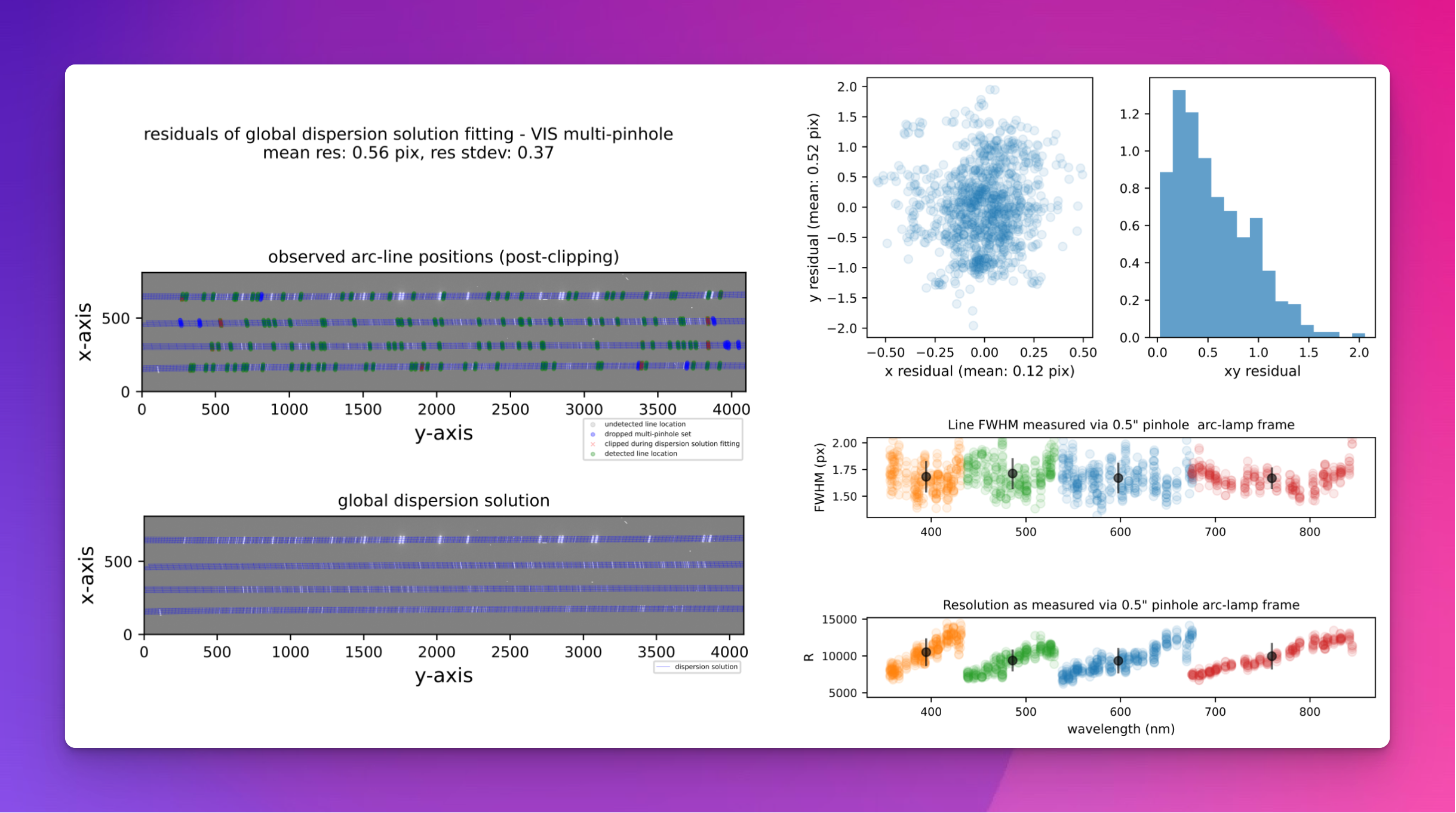
Fig. 48 A QC plot resulting from the soxs_spatial_solution recipe. The top-left panel shows an SOXS VIS arc-lamp frame, taken with a multi-pinhole mask. The green circles represent arc lines detected in the image, and the blue circles and red crosses are lines that were detected but dropped because other pinholes of the same arc line were not detected, or because the lines were clipped during polynomial fitting. The grey circles represent arc lines reported in the static calibration table that were not detected in the image. The bottom-left panel shows the same arc-lamp frame with the dispersion solution overlaid as a blue grid. Lines travelling along the dispersion axis (left to right) are lines of equal slit position, and lines travelling in the cross-dispersion direction (top to bottom) are lines of equal wavelength. The top-right panel shows the residuals of the dispersion solution fit, and the bottom-right panel shows the resolution measured for each line (projected through the pinhole mask), with different colours for each echelle order and the mean order resolution in black.

Recipe API

class soxs_spatial_solution(log, settings=False, inputFrames=[], verbose=False, overwrite=False, create2DMap=True, polyOrders=False, command=False, debug=False, turnOffMP=False)

Bases: soxspipe.recipes.base_recipe.base_recipe

Enhance the wavelength solution achieved with soxs_disp_solution by expanding the solution into the spatial dimension (along the slit)

Key Arguments

• log – logger

• settings – the settings dictionary

• inputFrames – input fits frames. Can be a directory, a set-of-files (SOF) file or a list of fits frame paths

• verbose – verbose. True or False. Default False

• overwrite – overwrite the product file if it already exists. Default False

• create2DMap – create the 2D image map of wavelength, slit-position and order from disp solution.

• polyOrders – the orders of the x-y polynomials used to fit the dispersion solution. Overrides parameters found in the yaml settings file. e.g 345435 is order_x=3, order_y=4 ,wavelength_x=5 ,wavelength_y=4, slit_x=3 ,slit_y=5. Default False.

• command – the command called to run the recipe

• debug – debug mode. True or False. Default False

• turnOffMP – turn off multiprocessing. True or False. Default False. If True, multiprocessing will be turned off and the recipe will run in serial. This is useful for debugging.

See produce_product method for usage.

Initialization

clean_up(forceFail=False)

clip_and_stack(frames, recipe, ignore_input_masks=False, post_stack_clipping=True)

detrend(inputFrame, master_bias=False, dark=False, master_flat=False, order_table=False)

flag_poor_data()

get_recipe_settings()

prepare_frames(save=False)

produce_product()

generate the 2D dispersion map

Return:

• productPath – the path to the 2D dispersion map

Usage

from soxspipe.recipes import soxs_spatial_solution
recipe = soxs_spatial_solution(
    log=log,
    settings=settings,
    inputFrames=fileList
)
disp_map = recipe.produce_product()

qc_median_flux_level(frame, frameType='MBIAS', frameName='master bias', medianFlux=False)

qc_ron(frameType=False, frameName=False, masterFrame=False, rawRon=False, masterRon=False)

report_output(rformat='stdout')

subtract_mean_flux_level(rawFrame)

update_fits_keywords(frame, rawFrames=False)

verify_input_frames()

verify input frames match those required by the soxs_spatial_solution recipe

If the fits files conform to the required input for the recipe, everything will pass silently; otherwise, an exception will be raised.

xsh2soxs(frame)