soxs_nod

The soxs_nod recipe reduces the science frames produced by the NTT and SOXS from a nodding mode observation block.

Input

Table 81 Input files for the soxs_nod recipe. The files are typically passed to the soxs_nod recipe via a set-of-file (sof) file listing one file per line.

Data Type	Content	Related OB
FITS Image	Raw science frames of targets observed in nodding mode	SOXS_slt_obs_AutoNodOnSlit, SOXS_slt_cal_TelluricStdNod, SOXS_slt_cal_SpecphotNod
FITS Image	Master flat frame (optional)	-
FITS Table	order location table containing coefficients to the polynomial fits describing the order locations.	-
FITS Table	Dispersion map table giving coefficients of polynomials describing 2D dispersion/spatial solution	-
FITS Image	Dispersion map FITS image with 3-extensions (wavelength, slit-position and echelle order number)	-

Table 82 Ancillary (static) files required by the soxs_nod recipe. These files are packaged with and shipped with the code.

Data Type	Content
FITS images	Default bad-pixel map
FITS Binary Table	A spectral format table for the detector, giving the minimum and maximum wavelengths covered by each spectral order.

Parameters

Table 83 The soxs_nod recipe parameters.

Parameter	Description	Type	Entry Point	Related Util
use_flat	divide image by master flat frame	bool	settings file	-
subtract_background	fit and subtract the intra-order background light	bool	settings file	-
save_single_frame_extractions	If True, each A and B stacked frame for each offset is saved as 2D image	bool	settings file	-
use_lacosmic	use la cosmic to remove CRHs before extraction	bool	settings file	-
stacked_clipping_sigma	the sigma clipping limit used when stacking frames into a composite frame	float	settings file	clip_and_stack
stacked_clipping_iterations	the maximum sigma-clipping iterations used when stacking frames into a composite frame	int	settings file	clip_and_stack
horne_extraction_slit_length	the length of the ‘slit’ used to collect object flux (in pixels). Doubles are boxcar extraction aperture size.	int	settings file	horne_extraction
horne_extraction_profile_poly_order	degree of the polynomial used to fit the dispersion-direction profiles of the object.	int	settings file	horne_extraction
horne_extraction_profile_global_clipping_sigma	sigma clipping limit when fitting the object profile (global over the order)	float	settings file	horne_extraction
horne_extraction_profile_clipping_sigma	sigma clipping limit when fitting the dispersion-direction profiles of the object	float	settings file	horne_extraction
horne_extraction_profile_clipping_iteration_count	maximum number of clipping iterations when fitting dispersion-direction profiles	int	settings file	horne_extraction
order_sample_count	number of cross-order slices per order	int	settings file	detect_continuum
slice_length	length of each slice (pixels)	int	settings file	detect_continuum
slice_width	width of each slice (pixels)	int	settings file	detect_continuum
peak_sigma_limit	height gaussian peak must be above median flux to be “detected” by code (std via median absolute deviation)	float	settings file	detect_continuum
order_deg	degree of order-component of global polynomial fit to object trace	int	settings file	detect_continuum
disp_axis_deg	degree of y-component of global polynomial fit to object trace	int	settings file	detect_continuum
poly_fitting_residual_clipping_sigma	clipping limit (median and mad) when fitting global polynomial to object trace	float	settings file	detect_continuum
poly_clipping_iteration_limit	maximum number of clipping iterations when fitting global polynomial to object trace	int	settings file	detect_continuum
background_subtraction: bspline_deg	degree of bsplines used to fit the inter-order background (if subtract_background == True)	int	settings file	subtract_background
background_subtraction: gaussian_blur_sigma	standard deviation of Gaussian kernel used to smooth background image (if subtract_background == True)	int	settings file	subtract_background
response: max_iteration	maximum number of iterations used to fit the polynomial to the response function	int	settings file	response_function
response: poly_order	degree of the polynomial used to fit the response function	int	settings file	response_function

Method

The algorithm used in the soxs_nod recipe is shown in Fig. 51.

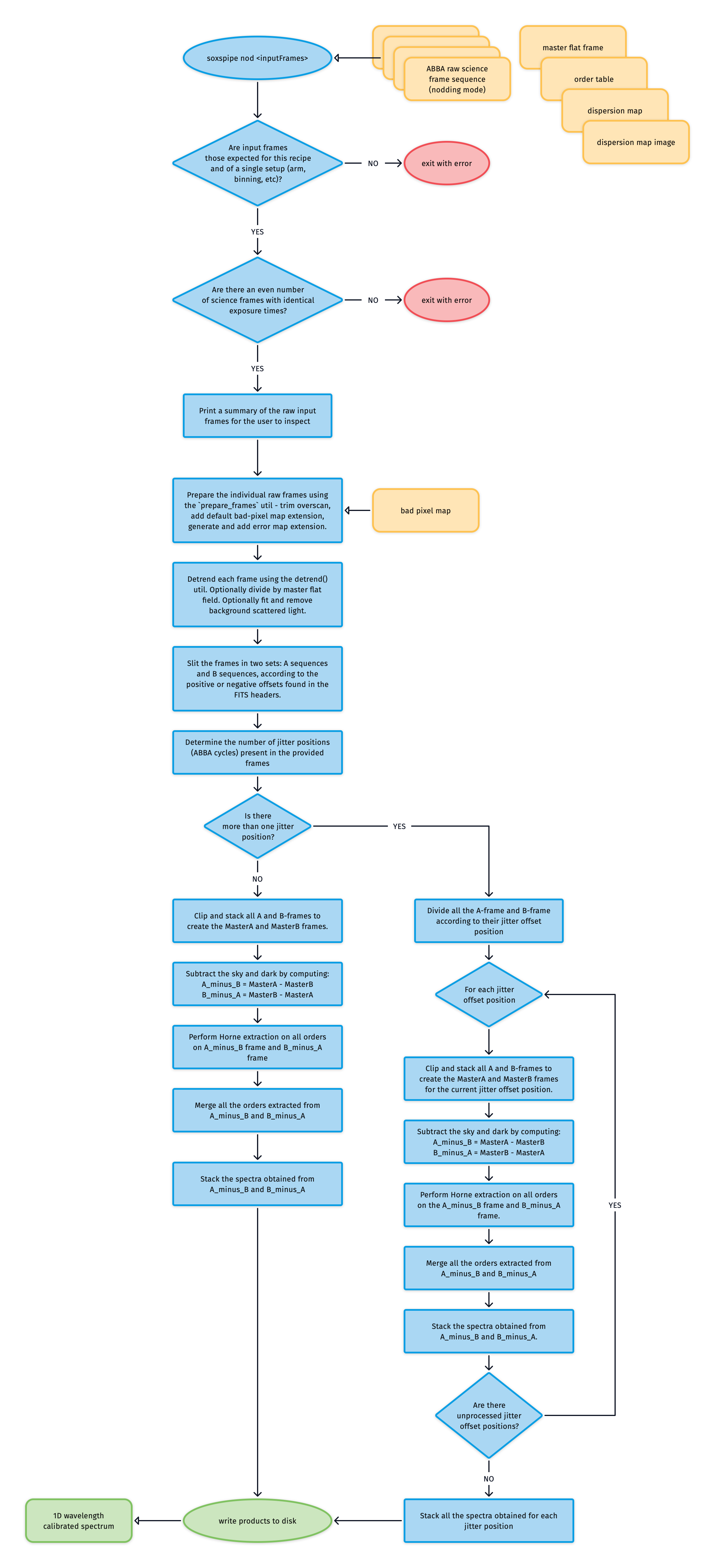
Fig. 51 The soxs_nod recipe reduced SOXS data acquired in nodding mode with one or multiple ABBA (jitter offsets) sequences.

During nodding observations, as described in the SOXS Observing Mode sections, 2 locations on the slit, A and B, separated by a few arcseconds, are considered. Observations are performed in pairs of equal-length exposures called cycles. First, a spectrum is taken with the target located at slit-position A. The telescope is then shifted, or ‘nodded’, so the target is at slit-position B and a second spectrum is taken. This process is then repeated in reverse to acquire the third and fourth exposures at slit-positions B and A, a BA cycle.

Two or more cycles are then combined into a sequence. The shortest sequence possible is AB and BA or ABBA, but sequences can be compiled by many cycles, e.g., an 8-cycle sequence ABBAABBAABBAABBA.

Within this schema, jittering can also be considered. In this case, the target is shifted by a slight random offset each time it is placed at slit positions A and B, avoiding putting the targets always on a bad row or column of the CCD. When including jitter an ABBA sequence becomes A \(^{1}\) B \(^{1}\) B \(^{2}\) A \(^{2}\), where the subscript indicates a location at the slit-positions A or B but now including a small random offset (a jitter).

Adopting this assumption, the soxs_nod recipe proceeds as follows. First, it identifies how many jitter positions are in the provided frames. If only one is present (in other words, no jitter offsets are considered), the recipe detrends the images using bias, flat field and subtracts the scattered background light. Then, all the frames in the A position are stacked together. The same is also done for frames in the B position. Then, two images, \(A - B\) and \(B - A\), are computed where A and B are the stacked images described before. Those images have the sky background and dark current subtracted. At this stage, the standard Horne extraction utility is run, and orders are extracted from the first and second subtracted images and merged. The two spectra obtained from the \(A - B\) and \(B - A\) images are stacked together for a unique spectrum.

If the jitter is present, the soxs_nod recipe determines how many different offsets are present in the provided frames, which are grouped according to their offsets before stacking. The procedure described above is then repeated for each offset detected in the input data. At the end of the procedure, there will be a number of spectra equal to the number of detected offsets in the data. Those spectra are then stacked and merged to obtain a unique spectrum.

Note a boxcar extraction is also preformed alongside the Horne extraction. Use the horne-extraction-slit-length to control the size of the aperture used to preform the boxcar extraction on the object trace.

Output

Table 84 Output files for the soxs_nod recipe and their respective ESO PRO keywords. Some output file may not be generated depending on the user’s pipeline settings.

Label	Content	Data Type	PRO CATG	PRO TYPE	PRO TECH
EXTRACTED ORDERS TABLE	Table of the extracted source in each order	FITS	SCI_SLIT_FLUX_NIR	REDUCED	ECHELLE,SLIT
EXTRACTED MERGED TABLE	Table of the extracted, order-merged	FITS	SCI_SLIT_FLUX_NIR	REDUCED	ECHELLE,SLIT
EXTRACTED FLUXCAL SPECTRUM	Table of the flux calibrated extracted spectrum	FITS	SCI_SLIT_FLUX_<ARM>	REDUCED	ECHELLE,SLIT
RESPONSE_FUNC	Response function coefficients	FITS	RESP_TAB_<ARM>	REDUCED	ECHELLE,SLIT
EFFICIENCY	Efficiency estimate	FITS	EFFICIENCY_TAB_<ARM>	REDUCED	ECHELLE,SLIT
EXTRACTED MERGED ASCII	Ascii version of extracted source spectrum	TXT	-	-	-
OBJECT TRACE RES	Residuals of the object trace polynomial fit	PDF	-	-	-
BKGROUND	Fitted intra-order image background	PDF	-	-	-
EXTRACTED ORDERS QC PLOT	QC plot of extracted source	PDF	-	-	-
EXTRACTED MERGED QC PLOT	QC plot of extracted order-merged source	PDF	-	-	-
EXTRACTED MERGED FLUXCALIBRATED QC PLOT	QC plot of extracted order-merged, flux-calibrated source	PDF	-	-	-
RESPONSE QC PLOT	Response curve QC plot.	PDF	-	-	-

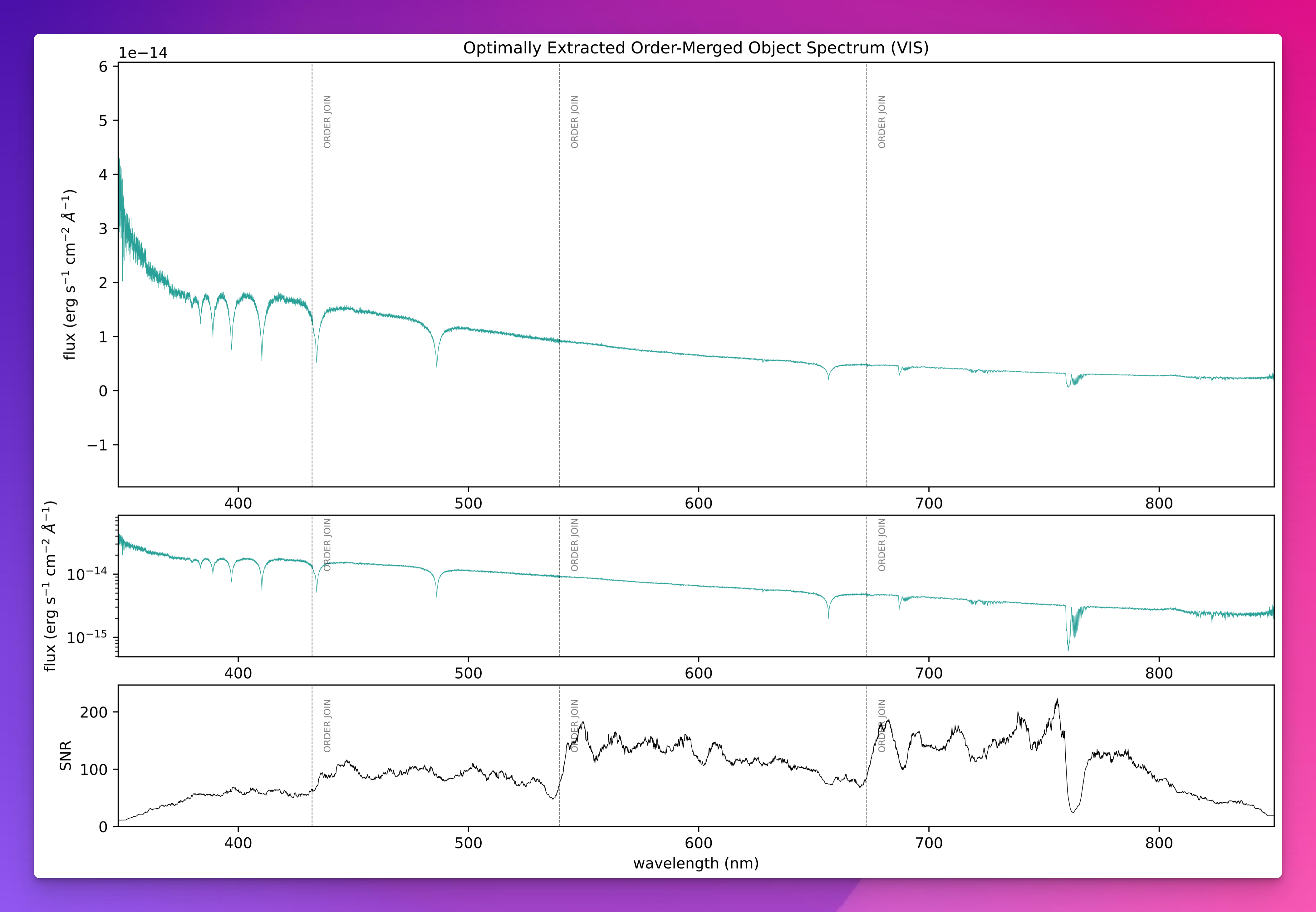
Fig. 52 A QC plot resulting from the soxs_nod recipe. This is a SOXS VIS wavelength and flux calibrated spectrum of the standard star CD-325613. The top- and middle-panels show the flux and wavelength calibrated spectrum, the top in linear-flux and the middle in log-flux scale. The bottom panel shows the signal-to-noise ratio across the entire wavelength range covered by the spectrum.

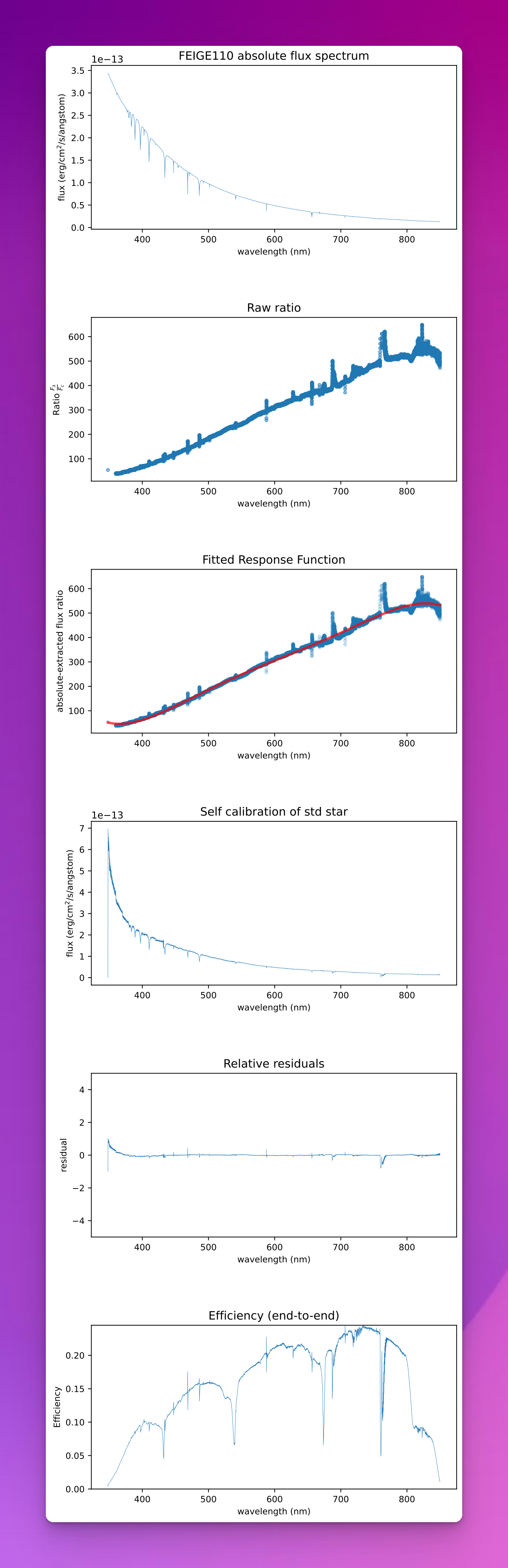
Fig. 53 The output of the reponse_function utility (used by nodding and stare recipes) used in the reduction of spectroscopic standard star spectra. The third panel shows th fittted response curve, and the final panel shows the overall efficiency of the instrument across the entire wavelength range of the spectrograph arm.

QC Metrics

Table 85 Quality Control metrics calculated in the soxs_nod recipe. Note that the acceptable ranges are enforced only for standard stars, not for science frames.

Label	Description	Unit	Acceptable Range
BADPIX FRAC	Fraction of bad pixels		VIS: [0.0,0.01], NIR: [-0.001,0.01]
INNER ORDER PIX MEAN	Mean inner-order pixel value	electrons	VIS: [-40,60], NIR: [-40,60]
INNER ORDER PIX SUM	Sum of all inner-order pixel values	electrons	-
BADPIX NUM	Number of bad pixels		-
N ORDERS	Number of orders containing an object trace		VIS: 4 , NIR: 15
SAMPLES DET NUM	Number of samples where a continuum is detected		-
SAMPLES DET FRAC	Fraction of samples where a continuum is detected		VIS: [0.93,1.0] NIR: [0.7,1.0]
SAMPLES TOT NUM	Total number of samples along orders		-
SAMPLES CLIP NUM	Number of continuum sample clipped during solution fitting		-
SAMPLES CLIP FRAC	Fraction of detected continuum samples clipped during solution fitting		VIS: [0.0,0.2], NIR: [0.0,0.3]
X RES MAX	Maximum residual in continuum fit along x-axis	px	-
X RES MIN	Minimum residual in continuum fit along x-axis	px	-
X RES SD	Std-dev of residual continuum fit along x-axis	px	VIS: [0.0,0.2]
Y RES MAX	Maximum residual in continuum fit along y-axis	px	-
Y RES MIN	Minimum residual in continuum fit along y-axis	px	-
Y RES SD	Std-dev of residual continuum fit along y-axis	px	NIR: [0.0,0.5]
EFF MEDIAN	The median efficiency (global)		VIS: [0.04,0.30], NIR: [0.02,0.2]
SNR MEDIAN	The median signal-to-noise ratio across all orders (global)		VIS: [50,1000], NIR: [7,200]
EFF MEDIAN O<N>	The median efficiency (order N)		-
SNR MEDIAN O<N>	The median signal-to-noise ratio across all orders (order N)		-

Recipe API

class soxs_nod(log, settings=False, inputFrames=[], verbose=False, overwrite=False, command=False, debug=False, turnOffMP=False, recipeName='soxs-nod')

Bases: soxspipe.recipes.base_recipe.base_recipe

Reduce SOXS/Xshooter data taken in nodding mode

Key Arguments

• log – logger

• settings – the settings dictionary

• inputFrames – input fits frames. Can be a directory, a set-of-files (SOF) file or a list of fits frame paths.

• verbose – verbose. True or False. Default False

• overwrite – overwrite the product file if it already exists. Default False

• command – the command called to run the recipe

• debug – generate debug plots. Default False

• turnOffMP – turn off multiprocessing. True or False. Default False. If True, multiprocessing will be turned off and the recipe will run in serial. This is useful for debugging.

• recipeName – the name of the recipe. Default “soxs-nod”. This is used to retrieve the recipe settings from the settings dictionary and to name the product file (soxs_offset inherits soxs_nod)

Usage

from soxspipe.recipes import soxs_nod
recipe = soxs_nod(
    log=log,
    settings=settings,
    inputFrames=fileList
).produce_product()

Initialization

clean_up(forceFail=False)

clip_and_stack(frames, recipe, ignore_input_masks=False, post_stack_clipping=True)

detrend(inputFrame, master_bias=False, dark=False, master_flat=False, order_table=False)

flag_poor_data()

get_recipe_settings()

prepare_frames(save=False)

process_single_ab_nodding_cycle(aFrame, bFrame, locationSetIndex, orderTablePath, notFlattened=False, masterFlat=False)

process a single AB nodding cycle

Key Arguments:

• aFrame – the frame taken at the A location. CCDData object.

• bFrame – the frame taken at the B location. CCDDate object.

• locationSetIndex – the index of the AB cycle

• orderTablePath – path to the order table

• notFlattened – if True, the extraction is performed on non-flattened data. Default False

• masterFlat – path to the master flat frame. Default False

Return:

• mergedSpectrumDF_A – the order merged spectrum of nodding location A (dataframe)

• mergedSpectrumDF_B – the order merged spectrum of nodding location B (dataframe)

Usage:

mergedSpectrumDF_A, mergedSpectrumDF_B = soxs_nod.process_single_ab_nodding_cycle(
    aFrame=aFrame, bFrame=bFrame, locationSetIndex=1, orderTablePath=orderTablePath, masterFlat=masterFlat)

produce_product()

The code to generate the product of the soxs_nod recipe

Return:

• productPath – the path to the final product

Usage

from soxspipe.recipes import soxs_nod
recipe = soxs_nod(
    log=log,
    settings=settings,
    inputFrames=fileList
)
nodFrame = recipe.produce_product()

qc_median_flux_level(frame, frameType='MBIAS', frameName='master bias', medianFlux=False)

qc_ron(frameType=False, frameName=False, masterFrame=False, rawRon=False, masterRon=False)

report_output(rformat='stdout')

stack_extractions(dataFrameList, notFlattened=False, orderJoins=None)

merge individual AB cycles into a master extraction

Key Arguments:

• dataFrameList – a list of order-merged spectrum dataframes

Return:

• stackedSpectrum – the combined spectrum in a dataframe

Usage:

stackedSpectrum = soxs_nod.stack_extractions(
    [mergedSpectrumDF_A, mergedSpectrumDF_B])

subtract_mean_flux_level(rawFrame)

update_fits_keywords(frame, rawFrames=False)

verify_input_frames()

verify the input frame match those required by the soxs_nod recipe

If the fits files conform to the required input for the recipe, everything will pass silently; otherwise, an exception will be raised.

xsh2soxs(frame)