soxs_order_centres

Starting with the first pass dispersion solution from the soxs_disp_solution recipe, the soxs_order_centres recipe finds and fits a global polynomial model to the central trace of each echelle order.

Usage

The soxs_order_centres recipe can be run with the following convention:

soxspipe [-Vx] order_centres <inputFrames> [-o <outputDirectory> -s <pathToSettingsFile> --poly=<ooww>]

To rerun a previously executed soxs_order_centres recipe, you can find the execution command at the end of the recipe log file (found in the workspace products/soxs_order_centres directory). Use the -x flag to overwrite the product files if they already exist. For example, from the root of your workspace, you would run a command like:

soxspipe order_centres sof/20251011T094554_VIS_1X1_1_OLOC_QTH_PINHOLE_10_0S_SOXS.sof -s ./sessions/base/soxspipe.yaml 

While the default polynomial fitting orders have been carefully tuned to robustly reduce most data, it is possible to execute this recipe while providing the order-trace polynomial fitting orders through the command line, with command line settings overriding those in the YAML settings file. For instance, to attempt a order trace fit using 3rd (x) and 6th-order (y) spectral-order (oo) component and a 4th-order (x) and 3rd-order (y) wavelength (ww) component:

soxspipe order_centres sof/20251011T094554_VIS_1X1_1_OLOC_QTH_PINHOLE_10_0S_SOXS.sof -s ./sessions/base/soxspipe.yaml  --poly=3643

To adjust the default settings for the soxs_order_centres recipe, open the soxspipe.yaml file referenced in the command above in a text editor, navigate to the soxs_order_centres dictionary, save the file and rerun the recipe command. The settings’ descriptions can be found in Table 13.

Product files are written in the products/soxs_order_centres, and QC plots are in the qc/soxs_order_centres workspace directory. A report of the product files, QC plots and metrics is also printed to the terminal. The QC metrics calculated for soxs_order_centres are found in soxs_order_centres_qc and a typical QC plot in soxs_order_centres_qc_fig.

Reduction Tips

If this recipe fails the order centre traces, the first parameter to adjust is poly-fitting-residual-clipping-sigma. Try reducing this to 3-5 sigma and rerun the recipe to see if a fit is found. If the fit still fails, next try and increase the slice-width to 5-9 pixels to give the code a better chance of detecting the trace.

You can also try adjusting the polynomial fitting orders in order-deg and disp-axis-deg. However, please be advised the pipeline itself will dynamically adjust these values if they fail to fit the default set. It will slowly reduce the orders and refit until it finds a fit or decides a fit can not be found (after five iterations of decreasing the orders).

Parameters

Table 13 The soxs_order_centres recipe parameters.

Parameter	Description	Type	Entry Point	Related Util
order_sample_count	number of cross-order slices per order	int	settings file	detect_continuum utility
slice_length	length of each slice (pixels)	int	settings file	detect_continuum utility
slice_width	width of each slice (pixels)	int	settings file	detect_continuum utility
peak_sigma_limit	height gaussian peak must be above median flux to be “detected” by code (std via median absolute deviation).	float	settings file	detect_continuum utility
disp_axis_deg	degree of y-component of global polynomial fit to order centres	int	settings file or command-line	detect_continuum utility
order_deg	degree of echelle order number component of global polynomial fit to order centres	int	settings file or command-line	detect_continuum utility
poly_fitting_residual_clipping_sigma	sigma clipping limit when fitting global polynomial to order centres	float	settings file	detect_continuum utility
poly_clipping_iteration_limit	maximum number of clipping iterations when fitting global polynomial to order centres	int	settings file	detect_continuum utility

Input

Table 14 Input files for the soxs_order_centres recipe. The files are typically passed to the soxs_order_centres recipe via a set-of-file (sof) file listing one file per line.

Data Type	Content	Related OB
FITS Image	Flat lamp through a single-pinhole mask	SOXS_slt_cal_VISLampFlatPinhole, SOXS_slt_cal_NIRLampFlatPinhole
FITS Image	Master Dark Frame (VIS only, optional)	-
FITS Image	Master Bias Frame (VIS only)	-
FITS Image	Dark frame (Lamp-Off) of equal exposure length as single-pinhole frame (Lamp-On) (NIR only)	SOXS_slt_cal_NIRLampFlatPinhole
FITS Table	First guess dispersion solution	-

Output

Table 15 Output files for the soxs_order_centres recipe and their respective ESO PRO keywords.

Label	Content	Data Type	PRO CATG	PRO TYPE	PRO TECH
ORDER CENTRES	Polynomial fits to the order centre traces	FITS	ORDER_TAB_<ARM>	REDUCED	ECHELLE,SLIT
ORDER CENTRES RES	Residuals of the order centre polynomial fit	PDF	-	-	-

QC Metrics

Table 16 Quality Control metrics calculated in the soxs_order_centres recipe.

Label	Description	Unit	Acceptable Range
N ORDERS	Number of order centre traces found		-
SAMPLES DET NUM	Number of samples where a continuum is detected		-
SAMPLES DET FRAC	Fraction of samples where a continuum is detected		VIS: [0.85,1.0], NIR: [0.80,1.0]
SAMPLES TOT NUM	Total number of samples along orders		-
SAMPLES CLIP NUM	Number of continuum sample clipped during solution fitting		-
SAMPLES CLIP FRAC	Fraction of detected continuum samples clipped during solution fitting		-
X RES MAX	Maximum residual in order centre fit along x-axis	px	-
X RES MIN	Minimum residual in order centre fit along x-axis	px	-
X RES SD	Std-dev of residual order centre fit along x-axis		VIS: [0,0.1]
Y RES MAX	Maximum residual in order centre fit along y-axis	px	-
Y RES MIN	Minimum residual in order centre fit along y-axis	px	-
Y RES SD	Std-dev of residual order centre fit along y-axis		NIR: [0,0.1]

Plots similar to the one below are generated after each execution of soxs_order_centres. The residuals of a ‘good’ fit typically have a mean and standard deviation of <0.2px.

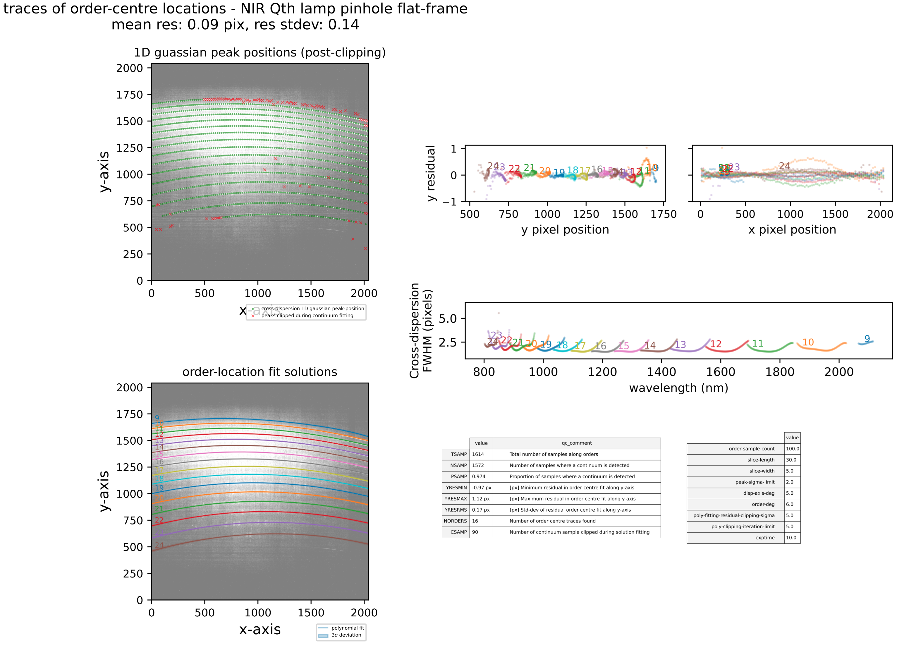
Fig. 14 A QC plot resulting from the soxs_order_centres recipe as run on a SOXS NIR single pinhole QTH flat lamp frame. The top-left panel shows the frame with green circles representing the locations on the cross-dispersion slices where a flux peak was detected. The red crosses indicate the centres of the slices where a peak was not detected. The bottom-left panel shows the global polynomial fitted to the detected order-centre trace with the different colours representing individual echelle orders. The top-right panels show the fit residuals in the X and Y axes. The bottom-right panel shows the FWHM of the trace fits (in pixels) as a function of echelle order and wavelength.