soxs_mflat

The soxs_mflat recipe creates a single normalised master-flat frame used to correct for non-uniformity in response to light across the detector plane. Hot and dead pixels are also detected and added to a bad-pixel mask. Finally, the echelle order edges are detected and fitted with a polynomial model.

Sources of this non-uniformity include: Varying pixel sensitivities. Obstructions in the optical path (e.g., dust or pollen grains). Vignetting at the edges of the detector. A flat frame is ideally an image taken with uniform illumination across the detector’s light-collecting pixels. This evenly exposed image can be used to identify irregularities in the detector’s response.

Input

Table 55 Input files for the soxs_mflat recipe. The files are typically passed to the soxs_mflat recipe via a set-of-file (sof) file listing one file per line.

Data Type	Content	Related OB	Min. Frame Count
FITS image	Raw flats frames (exposures with identical exposure time, slit-width and detectors readout parameters).	SOXS_slt_cal_NIRLampFlat, SOXS_slt_cal_NIRLampFlatAtt, SOXS_slt_cal_VISLampFlat, SOXS_slt_cal_VISLampFlatAtt	5
FITS Image	A master bias Frame (UV-VIS only)	-	-
FITS Image	A master dark frame or lamp-off frames with identical exposure times to the lamp-on flat frames (NIR only)	-	-
FITS Table	An order location table containing coefficients to the polynomial fit describing the order centre locations.	-	-

Table 56 Ancillary (static) files required by the soxs_mflat recipe. These files are packaged with and shipped with the code.

Data Type	Content
FITS images	Default bad-pixel map
FITS Binary Table	A spectral format table for the detector, giving the minimum and maximum wavelengths covered by each spectral order.

Parameters

Table 57 The soxs_mflat recipe parameters.

Parameter	Description	Type	Entry Point	Related Util
subtract_background	fit and subtract the intra-order background light	bool	settings file	subtract_background
stacked_clipping_sigma	the sigma clipping limit used when stacking frames into a composite frame	float	settings file	clip_and_stack
stacked_clipping_iterations	the maximum sigma-clipping iterations used when stacking frames into a composite frame	int	settings file	clip_and_stack
centre_order_window	size of the window (in pixels) used to measure flux in the central band to determine median exposure	int	settings file	-
slice_length_for_edge_detection	length of the cross_dispersion slices used to determine order edges	int	settings file	detect_order_edges
slice_width_for_edge_detection	width of the cross_dispersion slices used to determine order edges	int	settings file	detect_order_edges
min_percentage_threshold_for_edge_detection	minimum value flux can drop to as percentage of central flux and be counted as an order edge	int	settings file	detect_order_edges
max_percentage_threshold_for_edge_detection	maximum value flux can climb to as percentage of central flux and be counted as an order edge	int	settings file	detect_order_edges
disp_axis_deg	degree of y-component of global polynomial fit to order edges	int	settings file or command-line	detect_order_edges
order_deg	degree of echelle order number component of global polynomial fit to order edges	int	settings file or command-line	detect_order_edges
poly_fitting_residual_clipping_sigma	sigma clipping limit when fitting global polynomial to order edges	float	settings file	detect_order_edges
poly_clipping_iteration_limit	maximum number of clipping iterations when fitting global polynomial to order edges	int	settings file	detect_order_edges
low_sensitivity_clipping_sigma	pixels with a flux less than this many sigma (mad) below the median flux level added to the bp map	float	settings file	-
scale_d2_to_qth	scale d2 to qth lamp flats when stitching	bool	settings file	-
background_subtraction: bspline_deg	degree of bsplines used to fit the inter-order background (if subtract_background == True)	int	settings file	subtract_background
background_subtraction: gaussian_blur_sigma	Standard deviation of Gaussian kernel used to smooth background image (if subtract_background == True)	int	settings file	subtract_background

Method

The algorithm used in the soxs_mflat recipe is shown in Fig. 37.

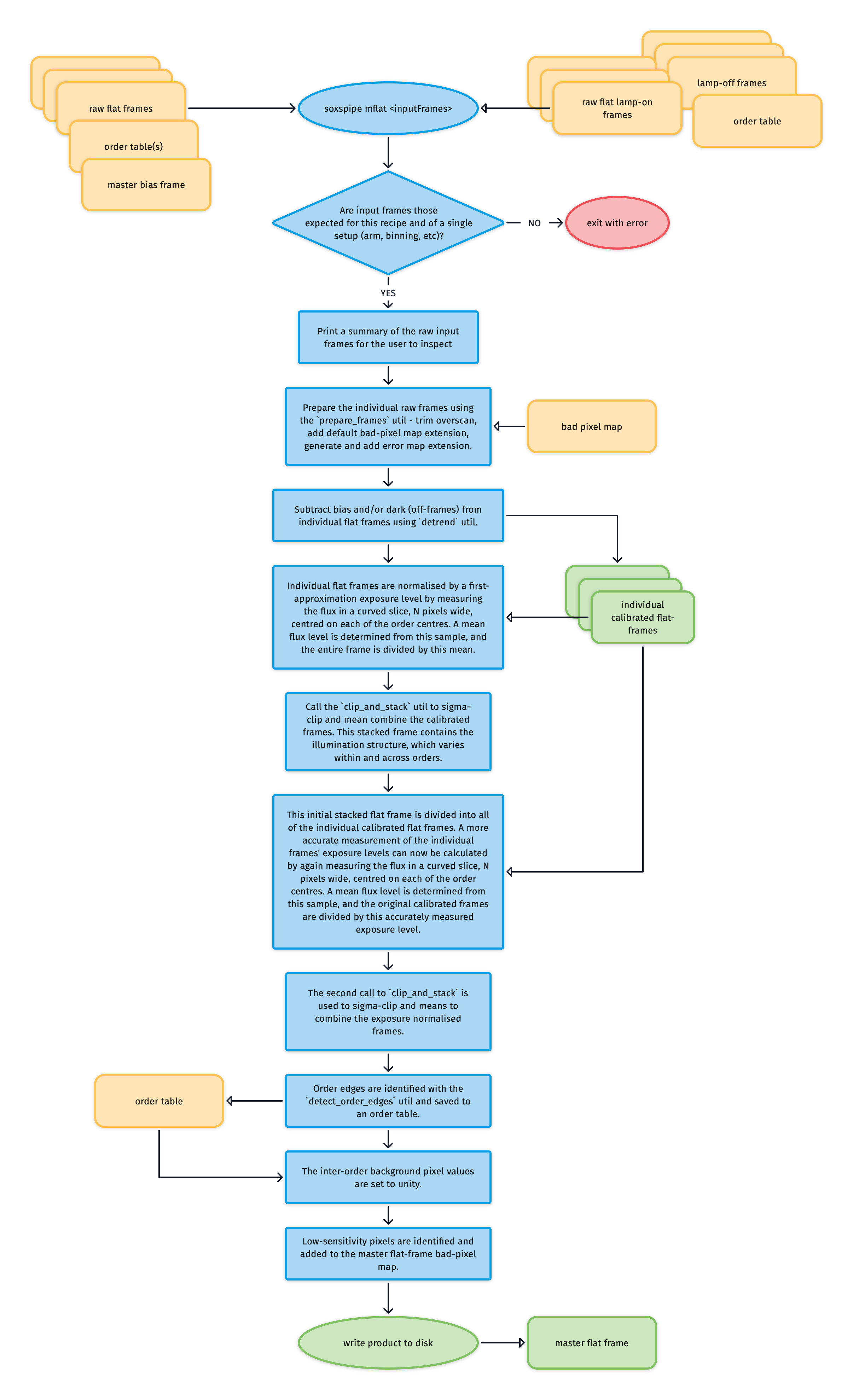
Fig. 37 The soxs_mflat recipe algorithm. At the top of the diagram, NIR input data is found on the right and VIS on the left.

The individual flat field frames have bias and dark signatures removed using the detrend utility. Here is an example of one such calibrated flat frame:

Normalising Exposure Levels in Individual Flat Frames

Once calibrated, exposure levels in the individual flat frames are normalised, as the total illumination varies from frame to frame. The individual frame exposure levels are calculated in two stages.

In the first stage, the mean inner-order pixel value across the frame is used as a first approximation of an individual frame’s exposure level. To calculate this mean value, the order locations identify a curved slice N pixels wide centred on each order centre, and bad pixels are masked (see Fig. 38). The collected inner-order pixel values are then sigma-clipped to exclude outlying values, and a mean value is calculated.

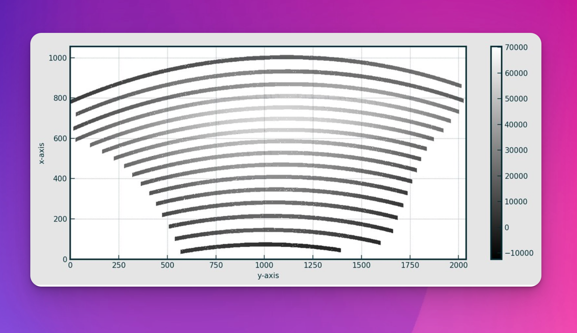
Fig. 38 The inner regions of the echelle orders are used to calculate a mean exposure level for the individual flats.

In a first attempt to normalise the exposure levels of individual frames, they are divided by their mean inner-order pixel value. These normalised flat frames are combined using the clip_and_stack utility to create a first-pass master-flat frame.

The second stage divides each original dark and bias-subtracted flat frame by this first-pass master flat (see Fig. 39). This removes the typical cross-plane illumination. So now, the mean inner-order pixel value across the frame will better estimate each frame’s intrinsic exposure level.

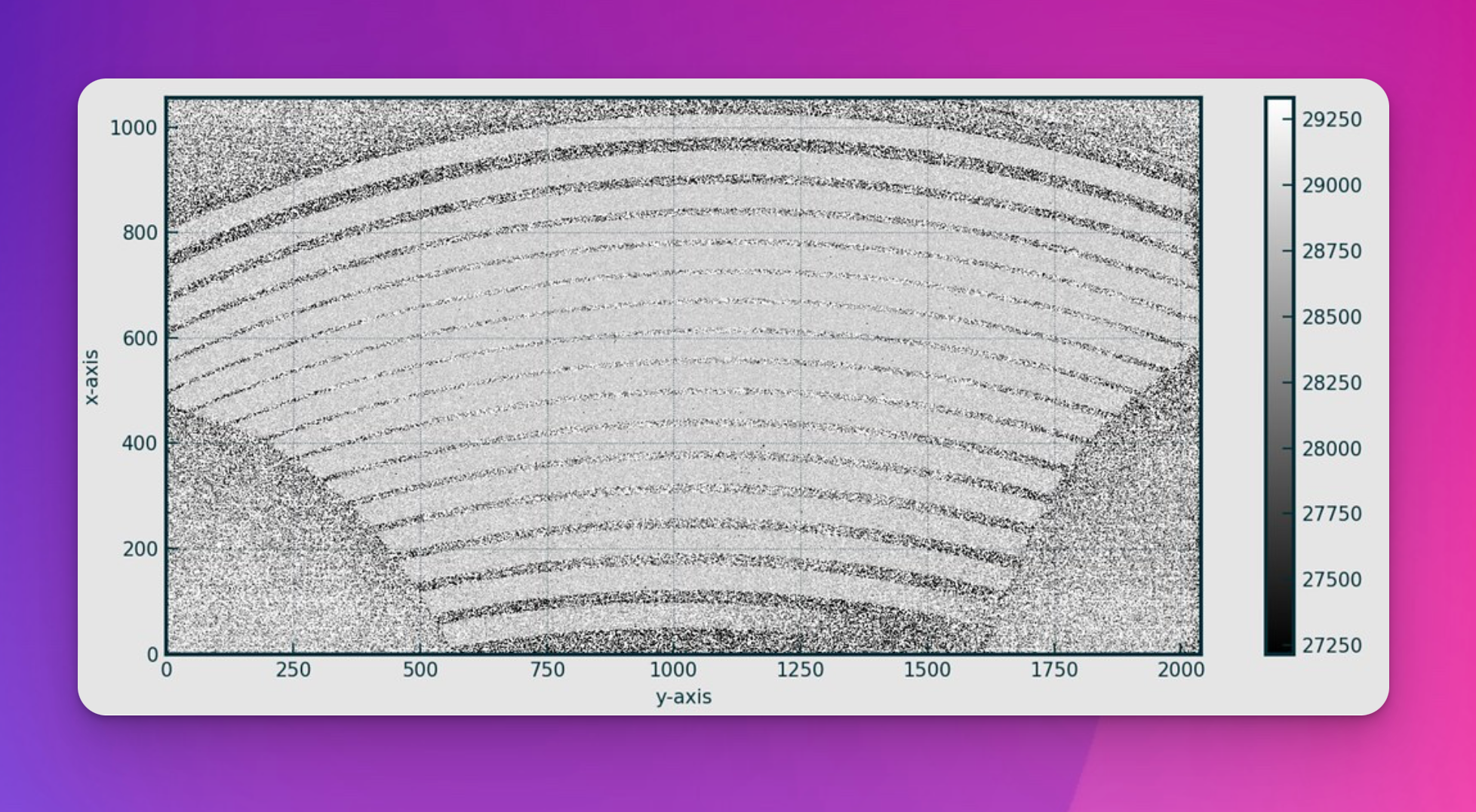
Fig. 39 An individual flat frame divided by the first-pass master flat.

On this frame, the mean inner-order pixel value is calculated again, and the original dark and bias-subtracted flat is re-normalised by being divided by this accurate measurement of its intrinsic exposure level.

Building a Final Master-Flat Frame

These re-normalised flats are then combined for a second time into a master-flat frame.

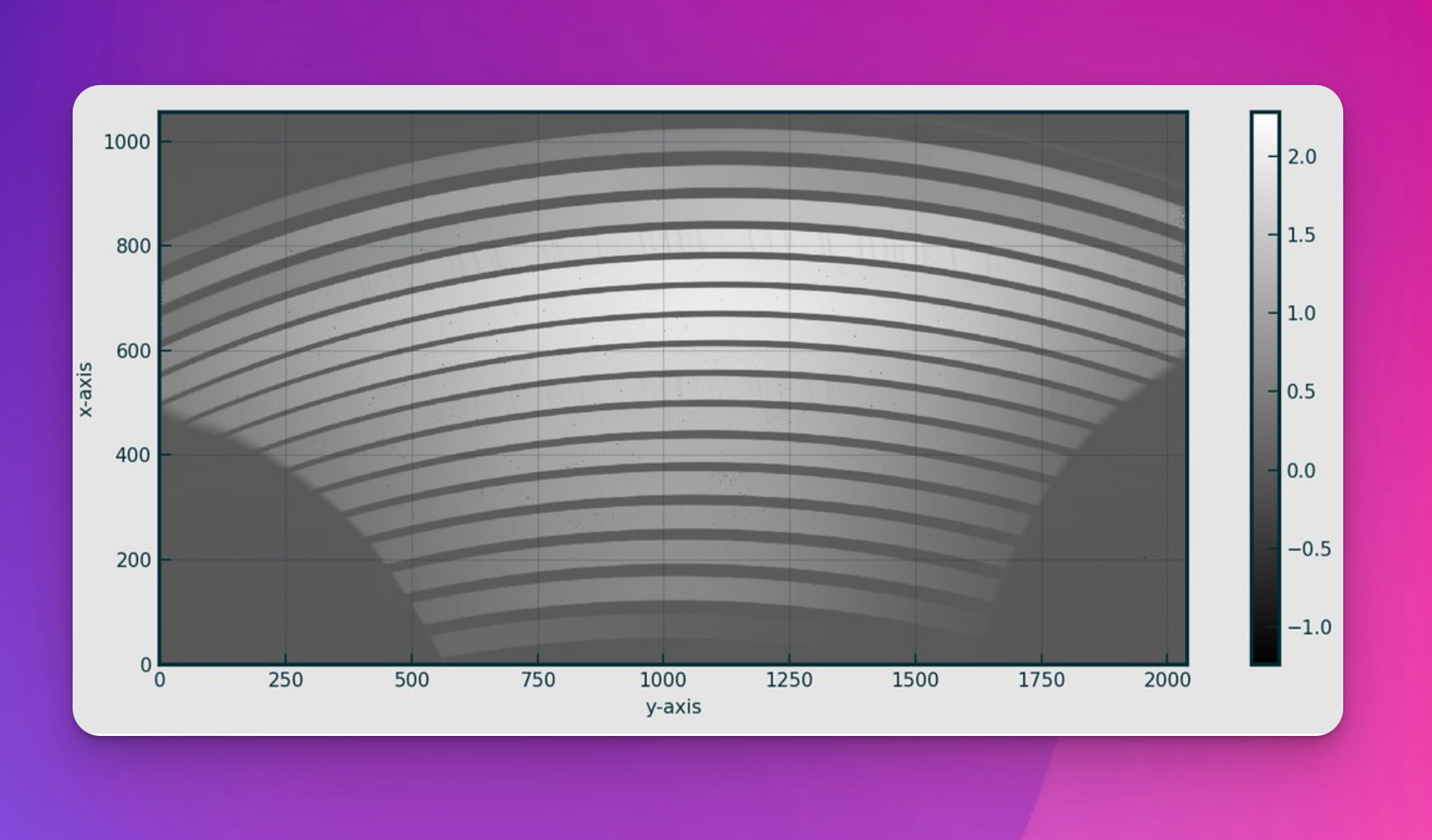
Fig. 40 A master-flat frame for Xshooter NIR.

Finally, order edges are located with the detect_order_edges utility, and the inter-order area pixel value is set to 1.

Low-sensitivity pixels are flagged and added to the bad-pixel map, and the final master-flat frame is written to disk.

UV Master Flat Frame Stitching

As the UV-VIS uses a combination of D-lamp and QTH-lamp flat sets, a further step is required to stitch the best orders from each of these master flats together into a dual-lamp master flat (see Fig. 41).

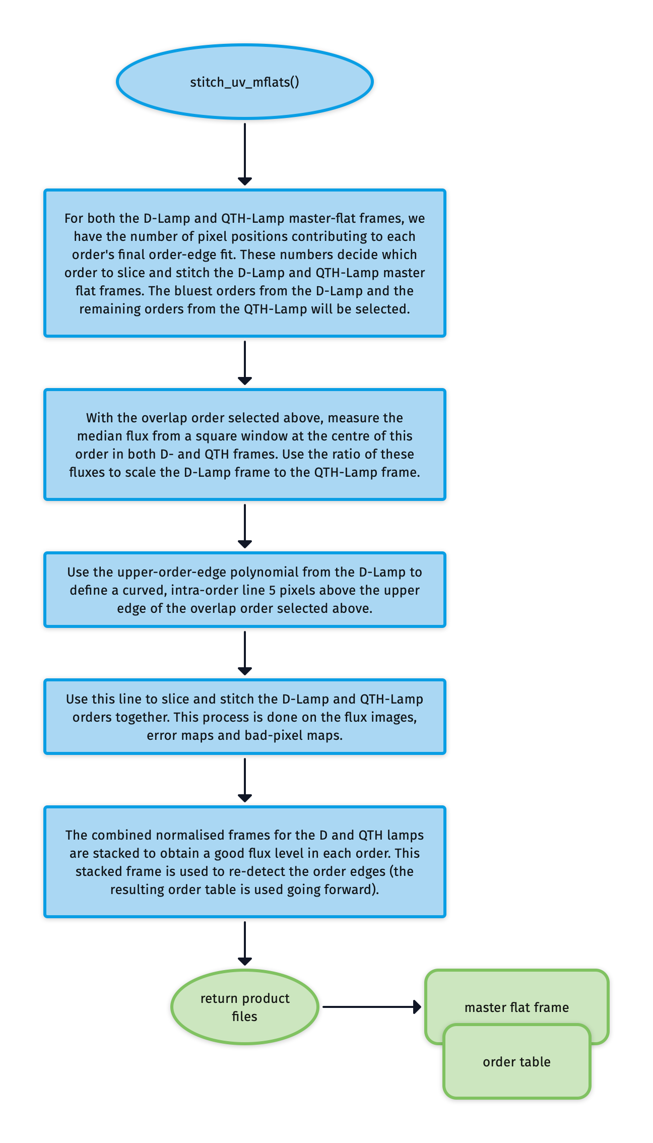
Fig. 41 The algorithm used to stitch together master flat frames from the UVB D- and QTH lamps to form a single flat frame covering the entire UVB wavelength range.

For both the D-Lamp and QTH-Lamp master flat frames, we have the number of pixel positions that contributed to the final order-edge fit for each order. We use these numbers to decide which orders to slice and stitch from the D-Lamp to the QTH-Lamp master flat frame.

With a crossover order now selected, the median flux from a square window at the centre of this order in both D- and QTH frames is measured. Using the ratio of these fluxes, the D-Lamp frame is scaled to the QTH-Lamp frame.

From the upper order-edge polynomial for the D-Lamp, we define a curved, intra-order line 5 pixels above the upper edge of the crossover order selected previously. This line is used to slice and stitch the D-Lamp and QTH-Lamp orders together. This process is done on the flux images, error maps and bad-pixel maps. Typically, the bluest orders from the D-Lamp will be selected, with the remaining orders coming from the QTH-Lamp.

Finally, the combined normalised frames for the D and QTH lamps are stacked to obtain a good flux level in each order. This stacked frame is used to re-detect the order edges (the resulting order table is used going forward).

Output

Table 58 Output files for the soxs_mflat recipe and their respective ESO PRO keywords (NIR and VIS).

Label	Content	Data Type	PRO CATG	PRO TYPE	PRO TECH
ORDER LOC	table of coefficients from polynomial fits to order locations	FITS	ORDER_TAB_<ARM>	REDUCED	ECHELLE,SLIT
MFLAT	master spectroscopic flat frame	FITS	MASTER_FLAT_<ARM>	REDUCED	IMAGE
ORDER LOC RES	visualisation of goodness of order edge fitting	PDF	-	-	-
BKGROUND	Fitted intra-order image background	PDF	-	-	-

Table 59 Output files for the soxs_mflat recipe for Xshooter UVB arm.

Label	Content	Data Type	PRO CATG	PRO TYPE	PRO TECH
ORDER LOC DLAMP	table of coefficients from polynomial fits to order locations	FITS	ORDER_TAB_<ARM>	REDUCED	ECHELLE,SLIT
MFLAT DLAMP	UVB master spectroscopic flat frame (DLAMP)	FITS	MASTER_FLAT_<ARM>	REDUCED	IMAGE
ORDER LOC QLAMP	table of coefficients from polynomial fits to order locations	FITS	ORDER_TAB_<ARM>	REDUCED	ECHELLE,SLIT
MFLAT QLAMP	UVB master spectroscopic flat frame (QLAMP)	FITS	MASTER_FLAT_<ARM>	REDUCED	IMAGE
ORDER LOC	table of coefficients from polynomial fits to order locations	FITS	ORDER_TAB_<ARM>	REDUCED	ECHELLE,SLIT
MFLAT	UVB master spectroscopic flat frame	FITS	MASTER_FLAT_<ARM>	REDUCED	IMAGE
ORDER LOC RES DLAMP	visualisation of goodness of order edge fitting	PDF	-	-	-
BKGROUND DLAMP	Fitted intra-order image background DLAMP	PDF	-	-	-
ORDER LOC RES QLAMP	visualisation of goodness of order edge fitting	PDF	-	-	-
BKGROUND QLAMP	Fitted intra-order image background QLAMP	PDF	-	-	-
ORDER LOC RES	visualisation of goodness of order edge fitting	PDF	-	-	-

QC Metrics

Table 60 Quality Control metrics calculated in the soxs_mflat recipe.

Label	Description	Unit	Acceptable Range
COLDPIX FRAC	Fraction of colf pixels		-
INNER ORDER PIX MEAN	Mean inner-order pixel value	electrons	VIS: [0.9,1.1], NIR: [0.9,1.1]
INNER ORDER PIX SUM	Sum of all inner-order pixel values	electrons	VIS: [100000,700000], NIR: [1000000,1200000]
COLDPIX NUM	Number of cold pixels		VIS: [0.0,0.01], NIR: [0.0,0.01]
N LOW SENS	Number of low-sensitivity pixels found in master flat	pixels	-
ORDEXP10	10th percentile inter-order flux	electrons	-
ORDEXP50	50th percentile inter-order flux	electrons	-
ORDEXP90	90th percentile inter-order flux	electrons	VIS: [10000,150000], NIR: [30000,60000]
X RES MAX	Maximum residual in order edge fit along x-axis	pixels	-
X RES MIN	Minimum residual in order edge fit along x-axis	pixels	-
X RES SD	Std-dev of residual order edge fit along x-axis	pixels	VIS: [0,0.37], NIR: [0,0.2]

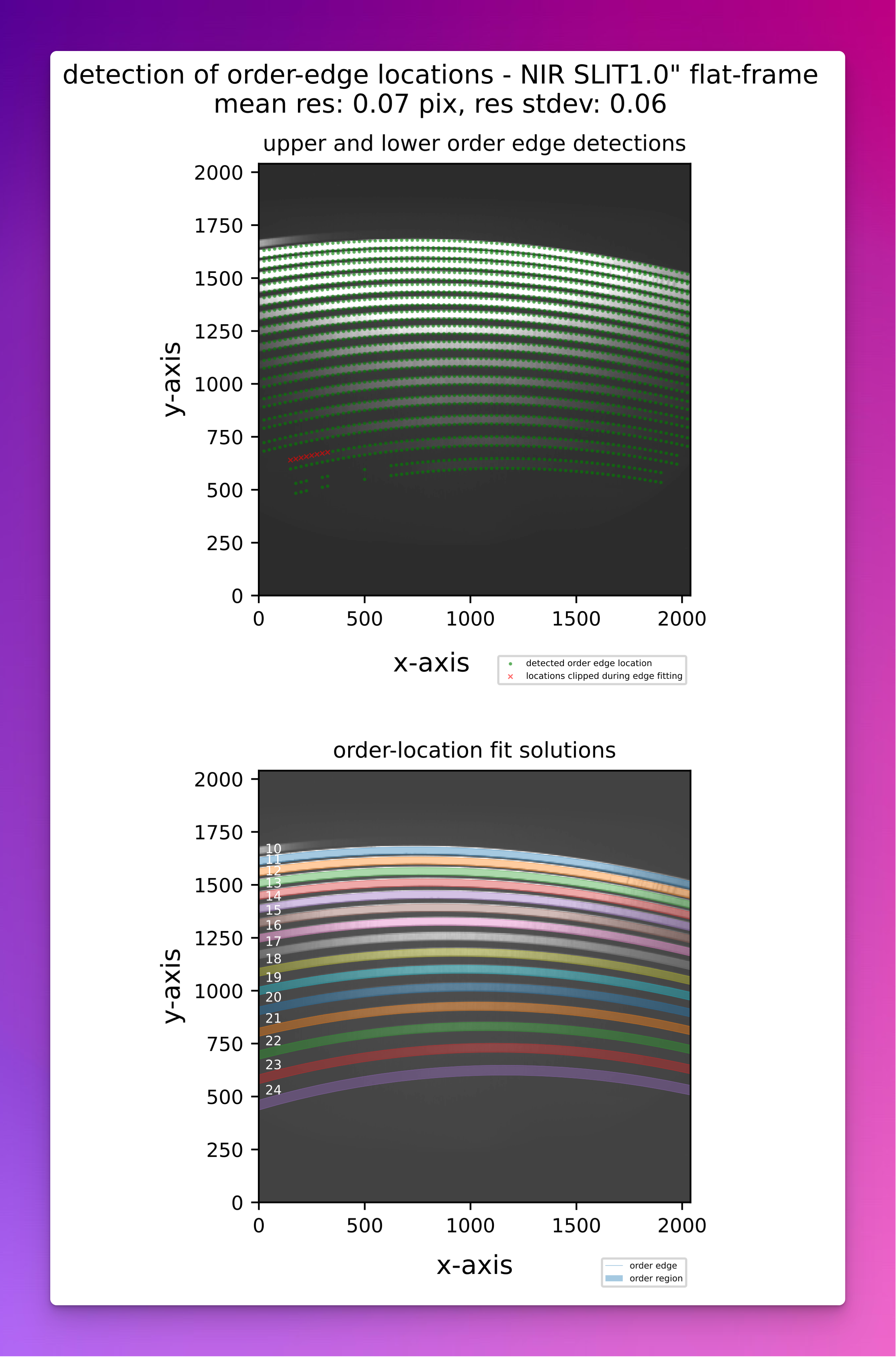
Fig. 42 A QC plot resulting from the soxs_mflat recipe (SOXS NIR). The top panel shows the upper and lower-order edge detections registered in the individual cross-dispersion slices in a SOXS NIR flat frame. The bottom panel shows the global polynomial fits to the upper and lower-order edges, with the area between the fits filled with different colours to reveal the unique echelle orders across the detector plane.

Recipe API

class soxs_mflat(log, settings=False, inputFrames=[], verbose=False, overwrite=False, command=False, debug=False, turnOffMP=False)

Bases: soxspipe.recipes.base_recipe.base_recipe

generate a single normalised master flat-field frame

Key Arguments

• log – logger

• settings – the settings dictionary

• inputFrames – input fits frames. Can be a directory, a set-of-files (SOF) file or a list of fits frame paths.

• verbose – verbose. True or False. Default False

• overwrite – overwrite the product file if it already exists. Default False

• command – the command called to run the recipe

• debug – generate debug plots. Default False

• turnOffMP – turn off multiprocessing. True or False. Default False. If True, multiprocessing will be turned off and the recipe will run in serial. This is useful for debugging.

Usage

from soxspipe.recipes import soxs_mflat
recipe = soxs_mflat(
    log=log,
    settings=settings,
    inputFrames=fileList
)
mflatFrame = recipe.produce_product()

Initialization

calibrate_frame_set()

given all of the input data calibrate the frames by subtracting bias and/or dark

Return:

• calibratedFlats – the calibrated frames

clean_up(forceFail=False)

clip_and_stack(frames, recipe, ignore_input_masks=False, post_stack_clipping=True)

detrend(inputFrame, master_bias=False, dark=False, master_flat=False, order_table=False)

find_uvb_overlap_order_and_scale(dcalibratedFlats, qcalibratedFlats)

find uvb order where both lamps produce a similar flux. This is the order at which the 2 lamp flats will be scaled and stitched together

Key Arguments:

• qcalibratedFlats – the QTH lamp calibration flats.

• dcalibratedFlats – D2 lamp calibration flats

Return:

• order – the order number where the lamp fluxes are similar

Usage:

overlapOrder = self.find_uvb_overlap_order_and_scale(dcalibratedFlats=dcalibratedFlats, qcalibratedFlats=qcalibratedFlats)

flag_poor_data()

get_recipe_settings()

mask_low_sens_pixels(frame, orderTablePath, returnMedianOrderFlux=False, writeQC=True)

add low-sensitivity pixels to bad-pixel mask

Key Arguments:

• frame – the frame to work on

• orderTablePath – path to the order table

• returnMedianOrderFlux – return a table of the median order fluxes. Default False.

• writeQC – add the QCs to the QC table?

Return:

• frame – with BPM updated with low-sensitivity pixels

• medianOrderFluxDF – data-frame of the median order fluxes (if returnMedianOrderFlux is True)

normalise_flats(inputFlats, orderTablePath, firstPassMasterFlat=False, lamp='')

determine the median exposure for each flat frame and normalise the flux to that level

Key Arguments:

• inputFlats – the input flat field frames

• orderTablePath – path to the order table

• firstPassMasterFlat – the first pass of the master flat. Default False

• lamp – a lamp tag for QL plots

Return:

• normalisedFrames – the normalised flat-field frames (CCDData array)

prepare_frames(save=False)

produce_product()

generate the master flat frames updated order location table (with egde detection)

Return:

• productPath – the path to the master flat frame

qc_median_flux_level(frame, frameType='MBIAS', frameName='master bias', medianFlux=False)

qc_ron(frameType=False, frameName=False, masterFrame=False, rawRon=False, masterRon=False)

report_output(rformat='stdout')

stitch_uv_mflats(medianOrderFluxDF, orderTablePath)

return a master UV-VIS flat frame after slicing and stitch the UV-VIS D-Lamp and QTH-Lamp flat frames

Key Arguments:

• medianOrderFluxDF – data frame containing median order fluxes for D and QTH frames

• orderTablePath – the original order table paths from order-centre tracing

Return:

• stitchedFlat – the stitch D and QTH-Lamp master flat frame

Usage:

mflat = self.stitch_uv_mflats(medianOrderFluxDF)

subtract_mean_flux_level(rawFrame)

update_fits_keywords(frame, rawFrames=False)

verify_input_frames()

verify the input frames match those required by the soxs_mflat recipe

If the fits files conform to required input for the recipe everything will pass silently, otherwise an exception will be raised.

xsh2soxs(frame)