soxs_disp_solution

The soxs_disp_solution recipe generates a first-guess dispersion solution for the instrument (measured along the central trace for each echelle order).

Input

Table 61 Input files for the soxs_disp_solution recipe. The files are typically passed to the soxs_disp_solution recipe via a set-of-file (sof) file listing one file per line.

Data Type	Content	Related OB
FITS Image	Arc Lamp through single pinhole mask	SOXS_slt_cal_VISArcsPinhole, SOXS_slt_cal_NIRArcsPinhole
FITS Image	Master Dark Frame (VIS only, optional)	-
FITS Image	Master Bias Frame (VIS only)	-
FITS Image	Dark frame (Lamp-Off) of equal exposure length as single pinhole frame (Lamp-On) (NIR only)	SOXS_slt_cal_NIRArcsPinhole

Table 62 Ancillary (static) files required by the soxs_disp_solution recipe. These files are packaged with and shipped with the code.

Data Type	Content
FITS images	Default bad-pixel map
FITS Binary Table	A spectral format table for the detector, giving the minimum and maximum wavelengths covered by each spectral order.
FITS Binary Table	An arc-lamp line list. This table gives the predicted x, y pixel position that each arc line is expected to appear near for each spectral order and pinhole in the multi-pinhole mask.

Parameters

Table 63 The soxs_disp_solution recipe parameters.

Parameter	Description	Type	Entry Point	Related Util
pixel_window_size	the size of the square window used to search for an arc-lamp emission line, centred on the predicted pixel position of the line	int	settings file	create_dispersion_map
pinhole_detection_thres_sigma	minimum significance required for arc-line to be considered ‘detected’	float	settings file	create_dispersion_map
order_deg	degree of echelle order number component of global polynomial fit to the dispersion solution [x, y]	int/list	settings file or command-line	create_dispersion_map
wavelength_deg	degree of wavelength component of global polynomial fit to the dispersion solution [x, y]	int/list	settings file or command-line	create_dispersion_map
poly_clipping_iteration_limit	number of sigma-clipping iterations to perform before settling on a polynomial fit for the dispersion solution	int	settings file	create_dispersion_map
poly_fitting_residual_clipping_sigma	sigma clipping limit when fitting global polynomial to the dispersion solution	float	settings file	create_dispersion_map

Method

After preparing and calibrating the single-pinhole arc-lamp frame, the create_dispersion_map) util is employed to detect and measure the positions of the arc lines on the frame. Once the line positions have been measured, a dispersion solution is generated by iteratively fitting a global polynomial against the observed line positions (see create_dispersion_map for details). The algorithm used in the soxs_disp_solution recipe is shown in Fig. 43. Note that saturated arc-lines are either absent from the input line-list file or get clipped during the fitting process and so are not included in the final dispersion solution fitting.

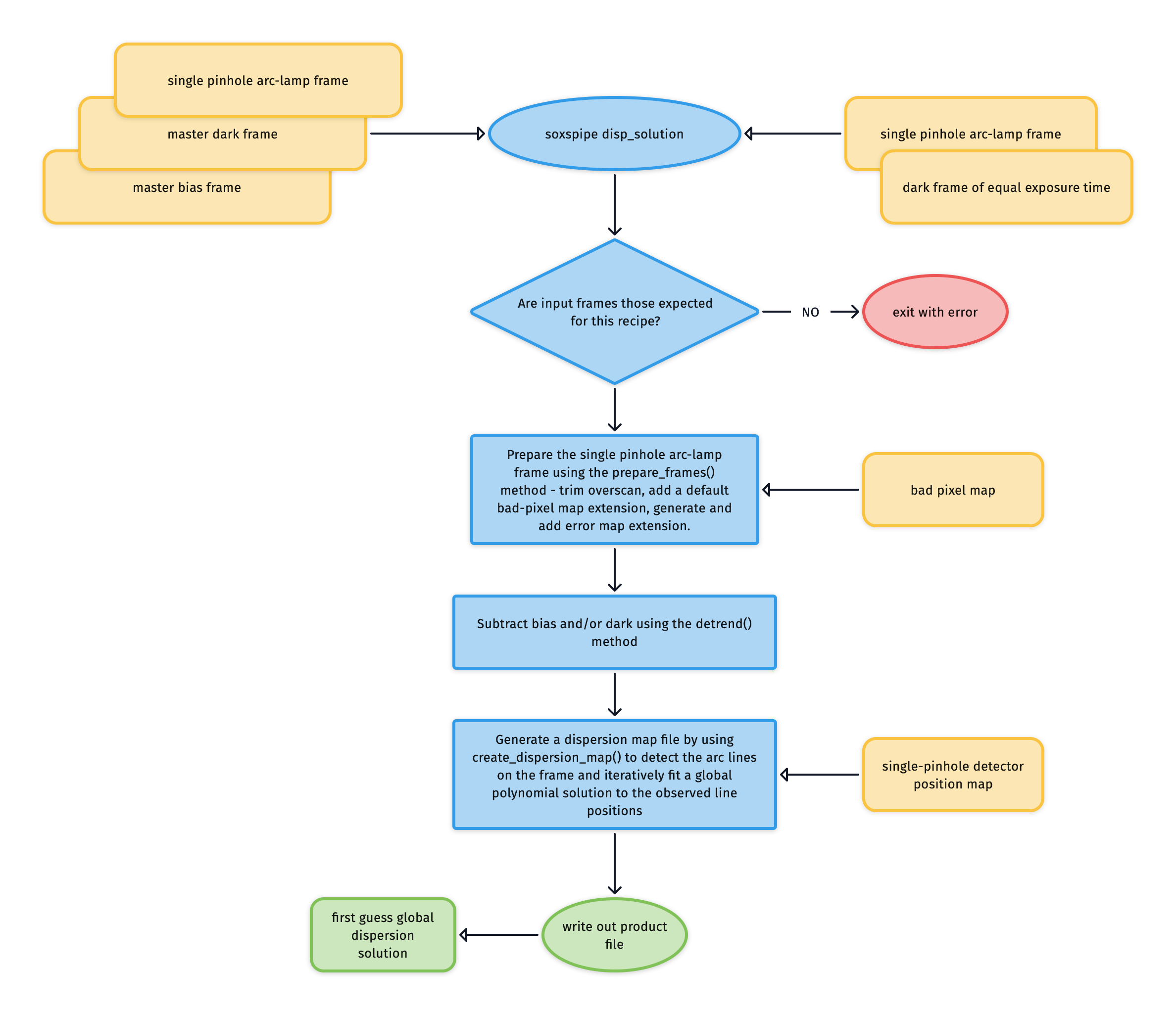
Fig. 43 The soxs_disp_solution recipe algorithm. At the top of the diagram, NIR input data is found on the right and VIS on the left.

Output

Table 64 Output files for the soxs_disp_solution recipe and their respective ESO PRO keywords.

Label	Content	Data Type	PRO CATG	PRO TYPE	PRO TECH
DISP MAP	first pass dispersion solution	FITS Table	DISP_TAB_<ARM>	REDUCED	ECHELLE,PINHOLE
DISP MAP LINES	dispersion solution fitted lines	FITS Table	-	-	-
DISP MAP LINES MISSING	undetected arc lines	FITS Table	-	-	-
DISP MAP RES	dispersion solution QC plots	PDF	-	-	-

QC Metrics

Table 65 Quality Control metrics calculated in the soxs_disp_solution recipe.

Label	Description	Unit	Acceptable Range
DETLINES CLIP NUM	Total number of detected lines clipped during solution fitting	lines	-
DETLINES NUM	Number of lines detected in single pinhole frame	lines	-
DETLINES FRAC	Proportion of input line-list lines detected on single pinhole frame		VIS: [0.9,1.0], NIR: [0.9,1.0]
DETLINES TOT	Total number of line in single line-list	lines	-
GOODLINES FRAC	Proportion of good, unclipped lines in single pinhole frame	lines	-
X RES MAX	Maximum residual in fitting of pinholes along x-axis (global)	pixels	-
X RES MIN	Minimum residual in fitting of pinholes along x-axis (global)	pixels	-
X RES MEDIAN	Median of absolute residuals in fitting of pinholes along x-axis (global)	pixels	VIS: [0.0,0.15], NIR: [0.0,0.35]
X RES SD	Std-dev of residuals in fitting of pinholes along x-axis (global)	pixels	VIS: [0,0.4], NIR: [0,1.0]
Y RES MAX	Maximum residual in fitting of pinholes along y-axis (global)	pixels	-
Y RES MIN	Minimum residual in fitting of pinholes along y-axis (global)	pixels	-
Y RES MEDIAN	Median of absolute residuals in fitting of pinholes along y-axis (global)	pixels	VIS: [0.0,0.9], NIR: [0.0,0.13]
Y RES SD	Std-dev of residuals in fitting of pinholes along y-axis (global)	pixels	VIS: [0,1.2], NIR: [0,0.25]
XY RES MAX	Maximum residual in fitting of pinholes (global)	pixels	-
XY RES MIN	Minimum residual in fitting of pinholes (global)	pixels	-
XY RES MEDIAN	Median residual in fitting of pinholes (global)	pixels	NIR: [0,1.0]
XY RES SD	Std-dev of residuals in fitting of pinholes (global)	pixels	VIS: [0,1.5], NIR: [0,1.0]
X DIFF MEDIAN	Median difference between observed and predicted pinhole detector locations along the x-axis (global)	pixels	-
X DIFF SD	Std-dev in difference between observed and predicted pinhole detector locations along the x-axis (global)	pixels	VIS: [0,3.0], NIR: [0,1.3]
Y DIFF MEDIAN	Median difference between observed and predicted pinhole detector locations along the y-axis (global)	pixels	-
Y DIFF SD	Std-dev in difference between observed and predicted pinhole detector locations along the y-axis (global)	pixels	VIS: [0,10.0], NIR: [0,1.5]
XY DIFF MEDIAN	Median difference between observed and predicted pinhole detector locations (global)	pixels	NIR: [0,6.0]
XY DIFF SD	Std-dev of difference between observed and predicted pinhole detector locations (global)	pixels	NIR: [0,1.9]
FWHM PIN MEDIAN	Median FWHM of detected lines in pinhole frames (global)	pixels	VIS: [1.60,1.75], NIR: [1.75,1.89]
FWHM PIN SD	Std-dev in FWHM of detected lines in pinhole frames (global)	pixels	VIS: [0.1,0.2], NIR: [0,0.211]
R PIN MEDIAN	Median spectral resolution measured from detected lines in pinhole frames (global)		-
X RES MAX O<N>	Maximum residual in fitting of pinholes along x-axis (order N)	pixels	-
X RES MIN O<N>	Minimum residual in fitting of pinholes along x-axis (order N)	pixels	-
X RES MEDIAN O<N>	Median of absolute residuals in fitting of pinholes along x-axis (order N)	pixels	-
X RES SD O<N>	Std-dev of residuals in fitting of pinholes along x-axis (order N)	pixels	-
Y RES MAX O<N>	Maximum residual in fitting of pinholes along y-axis (order N)	pixels	-
Y RES MIN O<N>	Minimum residual in fitting of pinholes along y-axis (order N)	pixels	-
Y RES MEDIAN O<N>	Median of absolute residuals in fitting of pinholes along y-axis (order N)	pixels	-
Y RES SD O<N>	Std-dev of residuals in fitting of pinholes along y-axis (order N)	pixels	-
XY RES MAX O<N>	Maximum residual in fitting of pinholes (order N)	pixels	-
XY RES MIN O<N>	Minimum residual in fitting of pinholes (order N)	pixels	-
XY RES SD O<N>	Std-dev of residuals in fitting of pinholes along (order N)	pixels	-
X DIFF MEDIAN O<N>	Median difference between observed and predicted pinhole detector locations along the x-axis (order N)	pixels	-
X DIFF SD O<N>	Std-dev in difference between observed and predicted pinhole detector locations along the x-axis (order N)	pixels	-
Y DIFF MEDIAN O<N>	Median difference between observed and predicted pinhole detector locations along the y-axis (order N)	pixels	-
Y DIFF SD O<N>	Std-dev in difference between observed and predicted pinhole detector locations along the y-axis (order N)	pixels	-
XY DIFF MEDIAN O<N>	Median difference between observed and predicted pinhole detector locations (order N)	pixels	-
FWHM PIN MEDIAN O<N>	Median FWHM of detected lines in pinhole frames (order N)	pixels	-
FWHM PIN SD O<N>	Std-dev in FWHM of detected lines in pinhole frames (order N)	pixels	-
R PIN MEDIAN O<N>	Median spectral resolution measured from detected lines in pinhole frames (order N)		-

The typical solution for the soxs_disp_solution recipe has sub-pixel residuals.

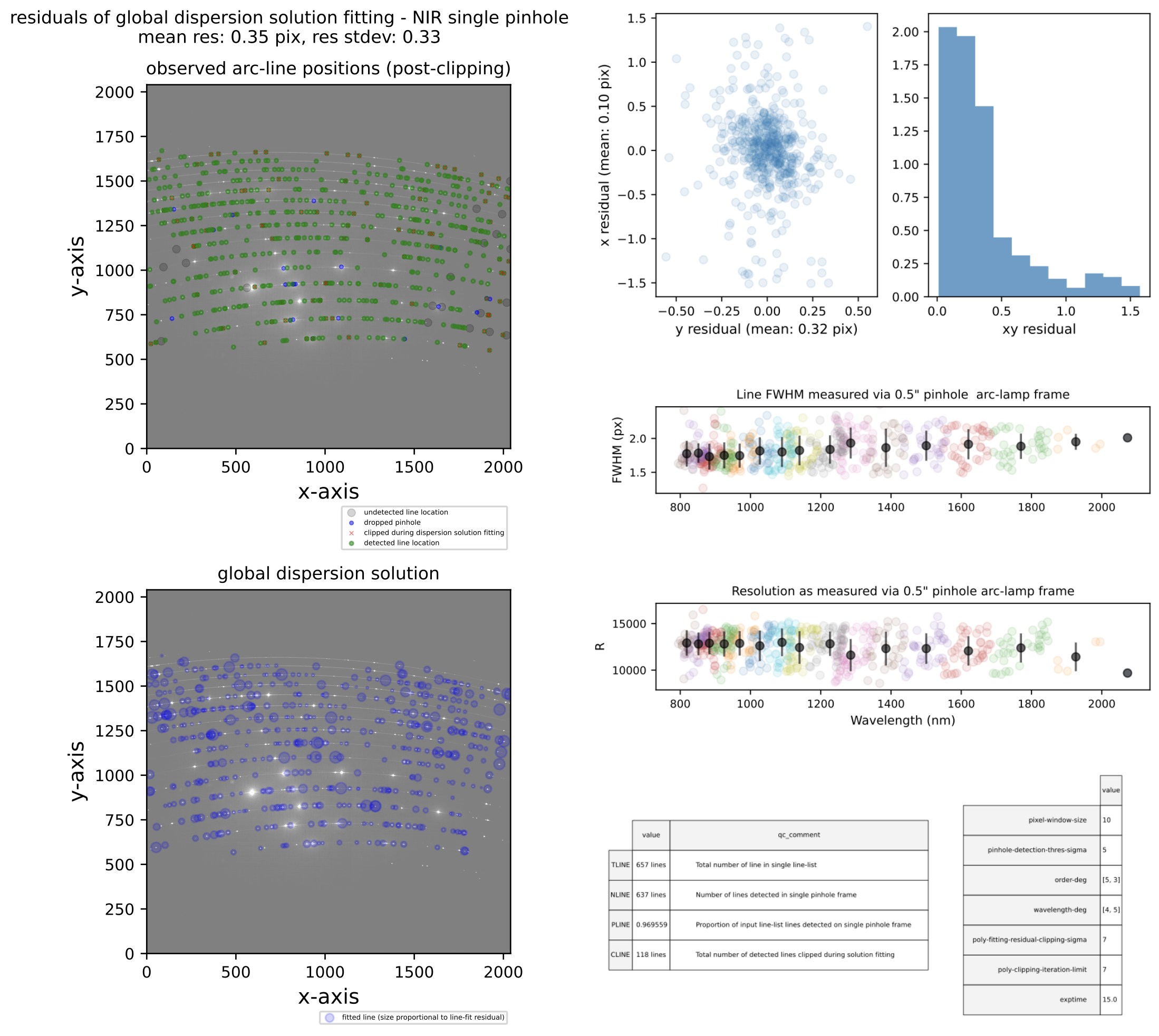
Fig. 44 A QC plot resulting from the soxs_disp_solution recipe as run on a SOXS NIR single pinhole arc lamp frame. A ‘good’ dispersion solution will have sub-pixel residuals (mean residuals \(<\) 0.5 pixels). The top-left panel shows an SOXS NIR arc-lamp frame, taken with a single pinhole mask. The green circles represent arc lines detected in the image, and the blue circles and red crosses were detected but dropped due to poor DAOStarFinder fitting or clipped during the polynomial fitting, respectively. The grey circles represent arc lines reported in the static calibration table that failed to be detected on the image. The bottom-left panel shows the same arc-lamp frame with the dispersion solution overlaid at the pixel locations modelled for the original lines in the line list. The top-right panels shows the residuals of the dispersion solution fit, and the final panels (bottom-right) the resolution measured for each line (as projected through the pinhole mask) with different colours for each echelle order and the mean order resolution in black.

Recipe API

class soxs_disp_solution(log, settings=False, inputFrames=[], verbose=False, overwrite=False, polyOrders=False, command=False, debug=False, turnOffMP=False)

Bases: soxspipe.recipes.base_recipe.base_recipe

generate a first approximation of the dispersion solution from single pinhole frames

Key Arguments

• log – logger

• settings – the settings dictionary

• inputFrames – input fits frames. Can be a directory, a set-of-files (SOF) file or a list of fits frame paths.

• verbose – verbose. True or False. Default False

• overwrite – overwrite the product file if it already exists. Default False

• polyOrders – the orders of the x-y polynomials used to fit the dispersion solution. Overrides parameters found in the yaml settings file. e.g 345400 is order_x=3, order_y=4 ,wavelength_x=5 ,wavelength_y=4. Default False.

• command – the command called to run the recipe

• debug – debug mode. True or False. Default False

• turnOffMP – turn off multiprocessing. True or False. Default False. If True, multiprocessing will be turned off and the recipe will run in serial. This is useful for debugging.

Usage

from soxspipe.recipes import soxs_disp_solution
disp_map_path = soxs_disp_solution(
    log=log,
    settings=settings,
    inputFrames=sofPath
).produce_product()

Initialization

clean_up(forceFail=False)

clip_and_stack(frames, recipe, ignore_input_masks=False, post_stack_clipping=True)

detrend(inputFrame, master_bias=False, dark=False, master_flat=False, order_table=False)

flag_poor_data()

get_recipe_settings()

prepare_frames(save=False)

produce_product()

generate a fisrt guess of the dispersion solution

Return:

• productPath – the path to the first guess dispersion map

qc_median_flux_level(frame, frameType='MBIAS', frameName='master bias', medianFlux=False)

qc_ron(frameType=False, frameName=False, masterFrame=False, rawRon=False, masterRon=False)

report_output(rformat='stdout')

subtract_mean_flux_level(rawFrame)

update_fits_keywords(frame, rawFrames=False)

verify_input_frames()

verify input frames match those required by the soxs_disp_solution recipe

If the fits files conform to the required input for the recipe, everything will pass silently; otherwise, an exception will be raised.

xsh2soxs(frame)