soxs_order_centres

Starting with the first pass dispersion solution from the soxs_disp_solution recipe, the soxs_order_centres recipe finds and fits a global polynomial model to the central trace of each echelle order.

Input

Table 66 Input files for the soxs_order_centres recipe. The files are typically passed to the soxs_order_centres recipe via a set-of-file (sof) file listing one file per line.

Data Type	Content	Related OB
FITS Image	Flat lamp through a single-pinhole mask	SOXS_slt_cal_VISLampFlatPinhole, SOXS_slt_cal_NIRLampFlatPinhole
FITS Image	Master Dark Frame (VIS only, optional)	-
FITS Image	Master Bias Frame (VIS only)	-
FITS Image	Dark frame (Lamp-Off) of equal exposure length as single-pinhole frame (Lamp-On) (NIR only)	SOXS_slt_cal_NIRLampFlatPinhole
FITS Table	First guess dispersion solution	-

Table 67 Ancillary (static) files required by the soxs_order_centres recipe. These files are packaged with and shipped with the code.

Data Type	Content
FITS images	Default bad-pixel map
FITS Binary Table	A spectral format table for the detector, giving the minimum and maximum wavelengths covered by each spectral order.

Parameters

Table 68 The soxs_order_centres recipe parameters.

Parameter	Description	Type	Entry Point	Related Util
order_sample_count	number of cross-order slices per order	int	settings file	detect_continuum utility
slice_length	length of each slice (pixels)	int	settings file	detect_continuum utility
slice_width	width of each slice (pixels)	int	settings file	detect_continuum utility
peak_sigma_limit	height gaussian peak must be above median flux to be “detected” by code (std via median absolute deviation).	float	settings file	detect_continuum utility
disp_axis_deg	degree of y-component of global polynomial fit to order centres	int	settings file or command-line	detect_continuum utility
order_deg	degree of echelle order number component of global polynomial fit to order centres	int	settings file or command-line	detect_continuum utility
poly_fitting_residual_clipping_sigma	sigma clipping limit when fitting global polynomial to order centres	float	settings file	detect_continuum utility
poly_clipping_iteration_limit	maximum number of clipping iterations when fitting global polynomial to order centres	int	settings file	detect_continuum utility

Method

The algorithm used in the soxs_order_centres recipe is shown in Fig. 45.

Once the single-pinhole flat-lamp frame has had the bias, dark and background subtracted it is passed to the detect_continuum utility to fit the order centres.

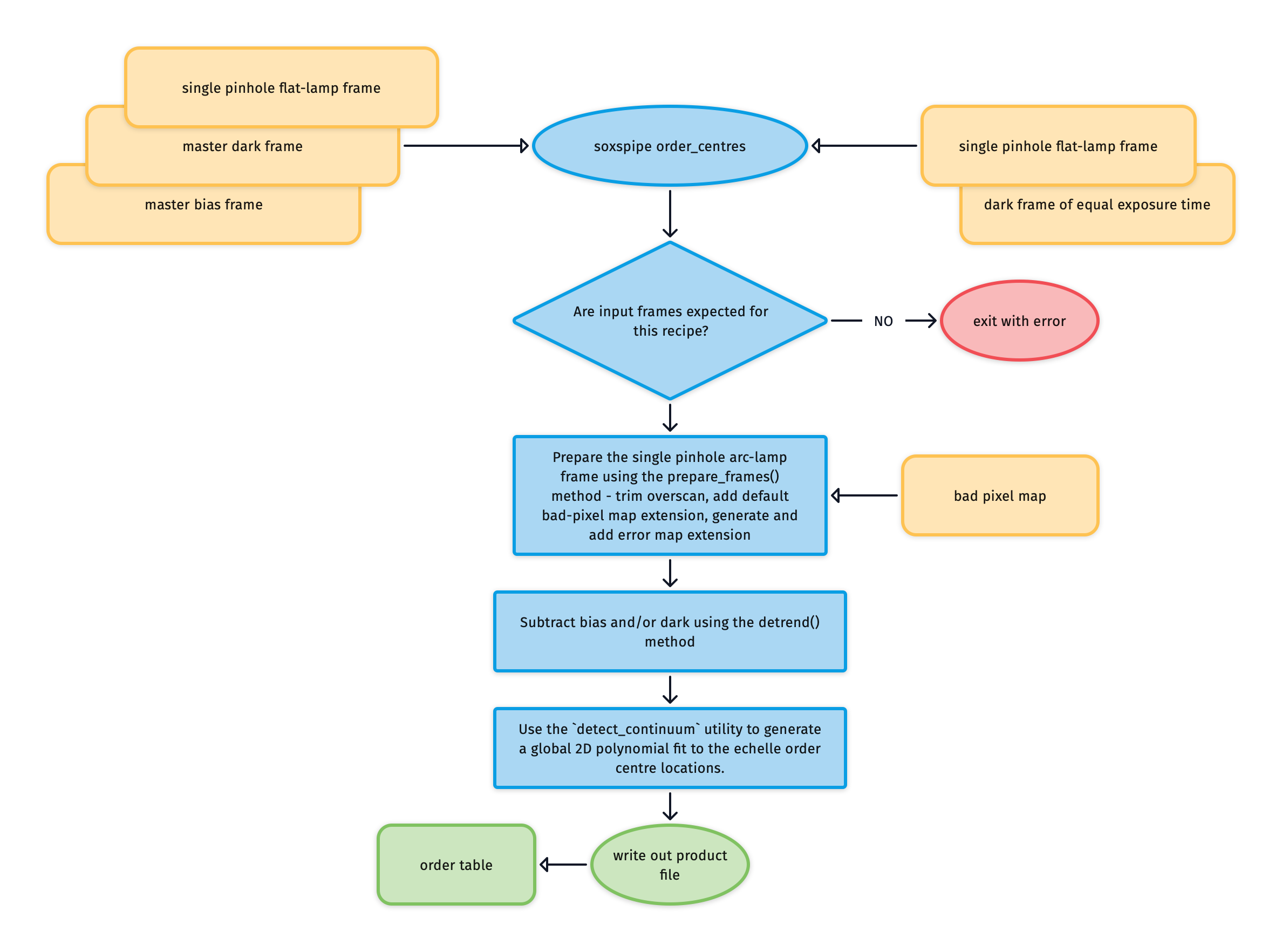
Fig. 45 The soxs_order_centres recipe algorithm. At the top of the diagram, NIR input data is found on the right and VIS on the left.

Output

Table 69 Output files for the soxs_order_centres recipe and their respective ESO PRO keywords.

Label	Content	Data Type	PRO CATG	PRO TYPE	PRO TECH
ORDER CENTRES	Polynomial fits to the order centre traces	FITS	ORDER_TAB_<ARM>	REDUCED	ECHELLE,SLIT
ORDER CENTRES RES	Residuals of the order centre polynomial fit	PDF	-	-	-

QC Metrics

Table 70 Quality Control metrics calculated in the soxs_order_centres recipe.

Label	Description	Unit	Acceptable Range
N ORDERS	Number of order centre traces found		-
SAMPLES DET NUM	Number of samples where a continuum is detected		-
SAMPLES DET FRAC	Fraction of samples where a continuum is detected		VIS: [0.85,1.0], NIR: [0.80,1.0]
SAMPLES TOT NUM	Total number of samples along orders		-
SAMPLES CLIP NUM	Number of continuum sample clipped during solution fitting		-
SAMPLES CLIP FRAC	Fraction of detected continuum samples clipped during solution fitting		-
X RES MAX	Maximum residual in order centre fit along x-axis	px	-
X RES MIN	Minimum residual in order centre fit along x-axis	px	-
X RES SD	Std-dev of residual order centre fit along x-axis		VIS: [0,0.1]
Y RES MAX	Maximum residual in order centre fit along y-axis	px	-
Y RES MIN	Minimum residual in order centre fit along y-axis	px	-
Y RES SD	Std-dev of residual order centre fit along y-axis		NIR: [0,0.1]

Plots similar to the one below are generated after each execution of soxs_order_centres. The residuals of a ‘good’ fit typically have a mean and standard deviation <0.2px.

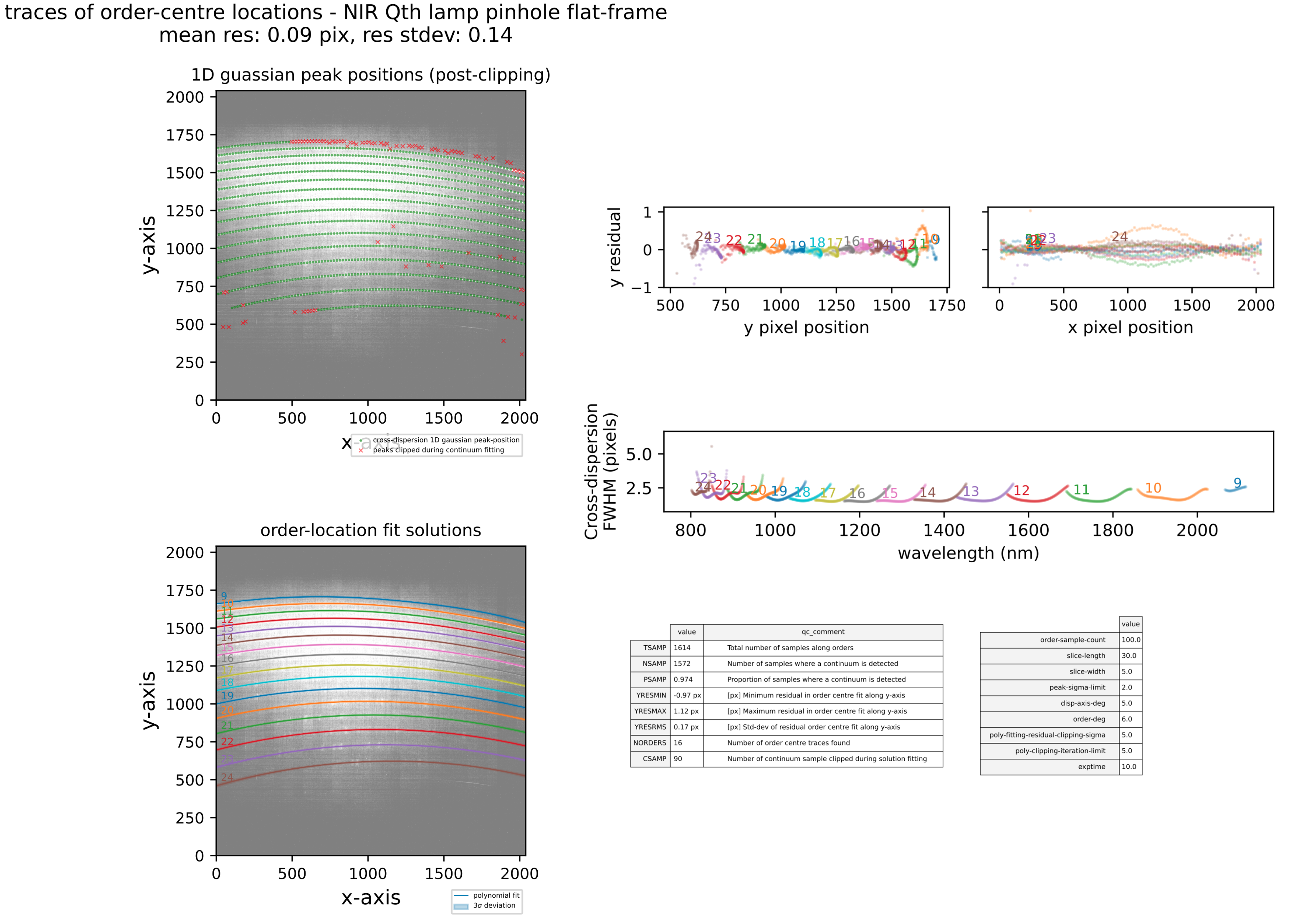
Fig. 46 A QC plot resulting from the soxs_order_centres recipe as run on a SOXS NIR single pinhole QTH flat lamp frame. The top-left panel shows the frame with green circles representing the locations on the cross-dispersion slices where a flux peak was detected. The red crosses show the centre of the slices where a peak failed to be detected. The bottom-left panel shows the global polynomial fitted to the detected order-centre trace with the different colours representing individual echelle orders. The top-right panels show the fit residuals in the X and Y axes. The bottom-right panel shows the FWHM of the trace fits (in pixels) with respect to echelle order and wavelength.

Recipe API

class soxs_order_centres(log, settings=False, inputFrames=[], verbose=False, overwrite=False, polyOrders=False, command=False, debug=False, turnOffMP=False)

Bases: soxspipe.recipes.base_recipe.base_recipe

further constrain the first guess locations of the order centres derived in soxs_disp_solution

Key Arguments

• log – logger

• settings – the settings dictionary

• inputFrames – input fits frames. Can be a directory, a set-of-files (SOF) file or a list of fits frame paths.

• verbose – verbose. True or False. Default False

• overwrite – overwrite the product file if it already exists. Default False

• polyOrders – the orders of the x-y polynomials used to fit the dispersion solution. Overrides parameters found in the yaml settings file. e.g 345400 is order_x=3, order_y=4 ,wavelength_x=5 ,wavelength_y=4. Default False.

• command – the command called to run the recipe

• debug – debug mode. True or False. Default False

• turnOffMP – turn off multiprocessing. True or False. Default False. If True, multiprocessing will be turned off and the recipe will run in serial. This is useful for debugging.

Usage

from soxspipe.recipes import soxs_order_centres
order_table = soxs_order_centres(
    log=log,
    settings=settings,
    inputFrames=a["inputFrames"]
).produce_product()

Initialization

clean_up(forceFail=False)

clip_and_stack(frames, recipe, ignore_input_masks=False, post_stack_clipping=True)

detrend(inputFrame, master_bias=False, dark=False, master_flat=False, order_table=False)

flag_poor_data()

get_recipe_settings()

prepare_frames(save=False)

produce_product()

generate the order-table with polynomal fits of order-centres

Return:

• productPath – the path to the order-table

qc_median_flux_level(frame, frameType='MBIAS', frameName='master bias', medianFlux=False)

qc_ron(frameType=False, frameName=False, masterFrame=False, rawRon=False, masterRon=False)

report_output(rformat='stdout')

subtract_mean_flux_level(rawFrame)

update_fits_keywords(frame, rawFrames=False)

verify_input_frames()

verify input frames match those required by the soxs_order_centres recipe

Return:

• None

If the fits files conform to the required input for the recipe, everything will pass silently; otherwise, an exception will be raised.

xsh2soxs(frame)